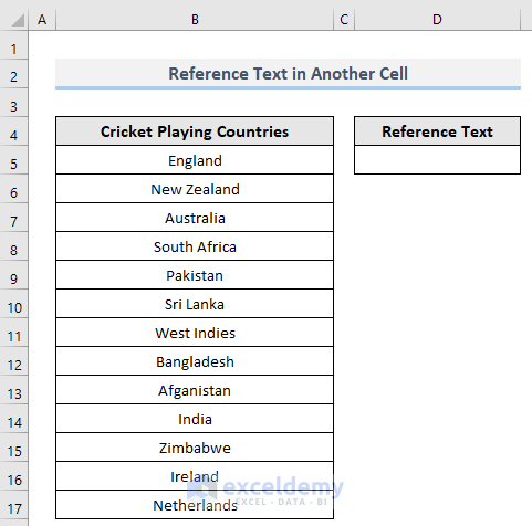
Method 1 – Reference Text from One Cell to Another Cell in the Same Worksheet in Excel
Consider the following example. We will take cell B7 and reference the text, Australia, from it in another cell, D5.
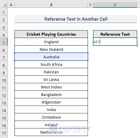
Steps:
- In cell D5, write an equal sign (=).
- Write the cell reference number, B7, that you want to cite in cell D5.
The formula will be like this:
=B7
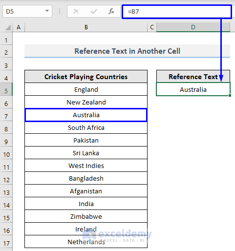
- Press Enter.
- Look at the following image for the result.
Read More: How to Display Text from Another Cell in Excel
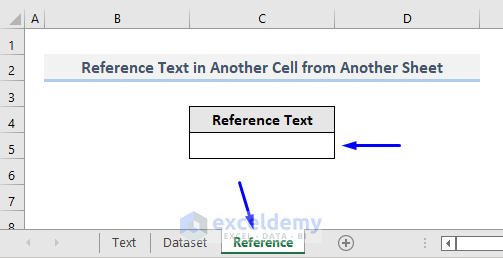
Method 2 – Citing Text from a Cell to Another Cell in Different Worksheet in Excel
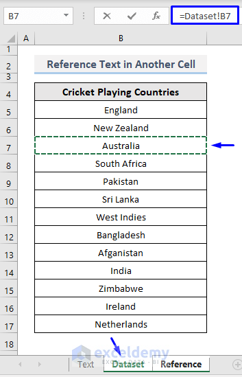
We have a list in the worksheet named Dataset (shown in the picture below).
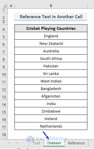
What we want to do here is refer to a specific text, Australia from cell B7, in cell C5 of the worksheet named Reference (shown in the picture below).
Steps:
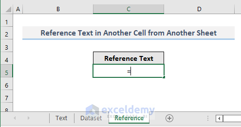
- In Cell C5 of the Reference worksheet, write an equal sign (=).
- Click on the Dataset sheet and select B7, the cell that you want to cite.
The formula will be like this:
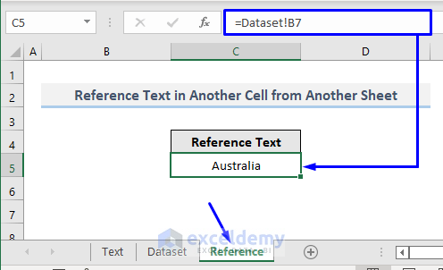
=Dataset!B7- Press Enter.
Look at the result shown in the picture below.
Read More: How to Use Variable Row Number as Cell Reference in Excel
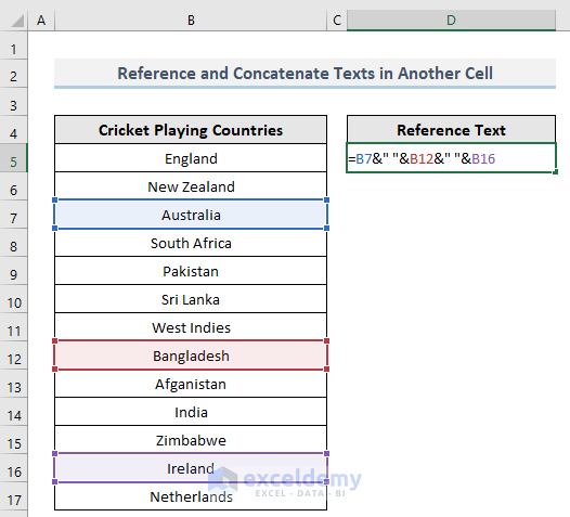
Method 3 – Referencing and Concatenating Texts in Another Cell
For this method, we will reference and concatenate Cells B7, B12 and B16 in Cell D5.
Steps:
- In Cell D5, write an equal sign (=).
- Write the cell reference numbers with ampersand symbol (&) between them.
The formula will be like this,
=B7&” “&B12&” “&B16The “ “ in between the ampersand symbol (&) is for spacing out among the referenced texts in cell D5. You can omit this if you don’t want to put space between texts.
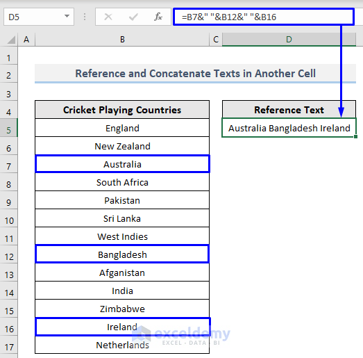
- Press Enter.
Look at the result shown in the picture below.
Read More: How to Reference Cell by Row and Column Number in Excel
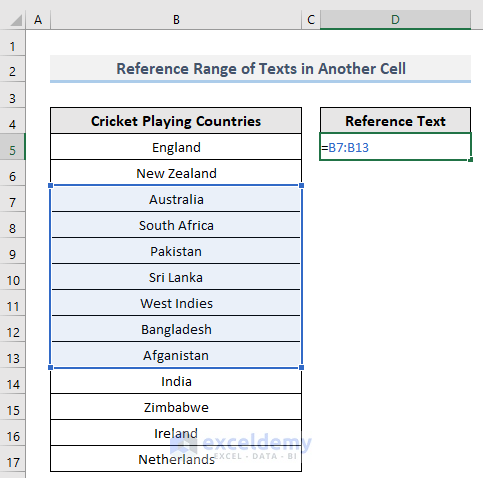
Method 4 – Reference a Range of Texts in Another Cell in Excel
Steps:
- In Cell D5, write an equal sign (=).
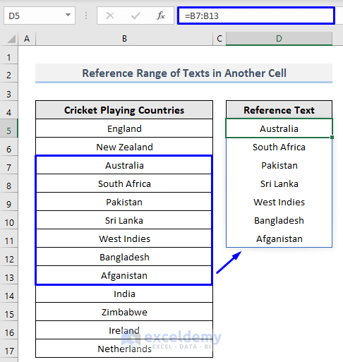
- Select the first cell from the range that you want to reference text from and drag through the last cell of the range. For instance, we wanted to reference text value from Australia (in Cell B7) to Afganistan (in Cell B13) in cell D5, so we selected cell B7 first and dragged to cell B13.
In cell D5, the formula looks like this:
=B7:B13- Press Enter.
To find out what happened, look at the image below.
Read More: How to Find and Replace Cell Reference in Excel Formula
Method 5 – Cite Text in Another Cell with Named Range in Excel
Steps:
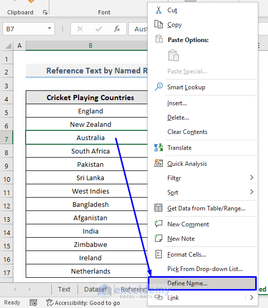
- Select the cell that you want to cite. In our case, it is cell B7.
- Right-click on the selected cell.
- Select Define Name… from the options.
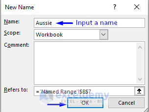
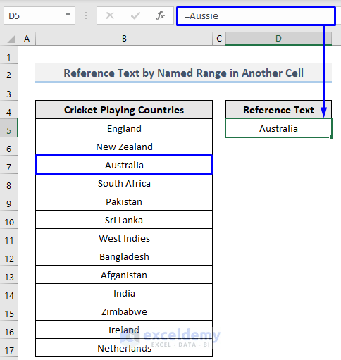
- A New Name pop-up box will appear. In the Name box, write any name that you like (we named our cell Aussie).
- Click OK.
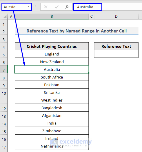
- We have successfully named the cell B7 Aussie (shown in the picture below).
- In cell D5, write an equal sign (=) and the newly defined name (Aussie).
The formula in cell D5 will be like this:
=Aussie- Press Enter.
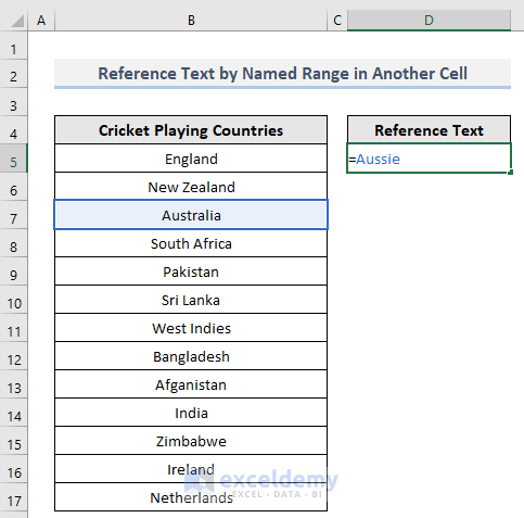
- Look at the following image to check that Excel referenced the text value Australia from cell B7 in cell D5.
Read More: How to Use Cell Value as Worksheet Name in Formula Reference in Excel
Method 6 – Reference Multiple Texts with Named Range in Another Cell
Steps:
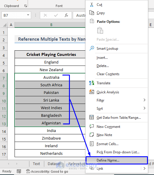
- Select the range of cells that you want to cite. In our case, we used cells B7 to B13.
- Right-click on the selected cells.
- Select Define Name… from the options.
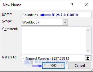
- A New Name pop-up box will appear. In the Name box, write any name that you like (we named our range Countries).
- Click OK.
- We have successfully named the range B7:B13 Countries (shown in the picture below).
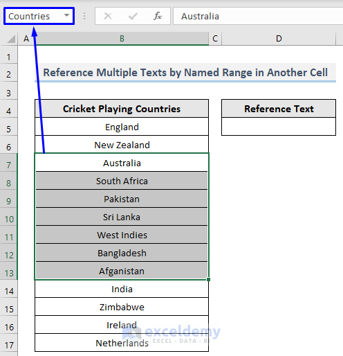
- In cell D5, write an equal sign (=) and the newly defined name (Countries).
The formula in cell D5 will be like this:
=Countries- Press Enter.
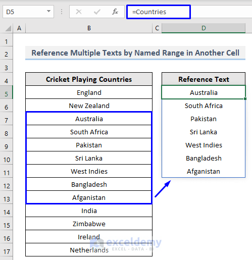
- Excel referenced the text value from Australia to Afganistan from cell B7 to B13 in cell D5.
Read More: How to Use OFFSET for Cell Reference in Excel
Method 7 – Reference Text from a Cell to Another Cell in the Same Worksheet with the INDIRECT Function
- Syntax:
=INDIRECT(ref_text, [a1])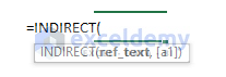
- Return Value:
Returns the reference value specified by a text string.
- Parameter Description:
| Parameter | Required/ Optional | Description |
|---|---|---|
| ref_text | Required | A reference of a cell containing an A1-style reference, an R1C1-style reference, a name defined as a reference, a text string as a reference.
The INDIRECT function will return the #REF! Error, if:
|
| [a1] | Optional | A logical value that determines the type of reference stored in the ref_text range.
|
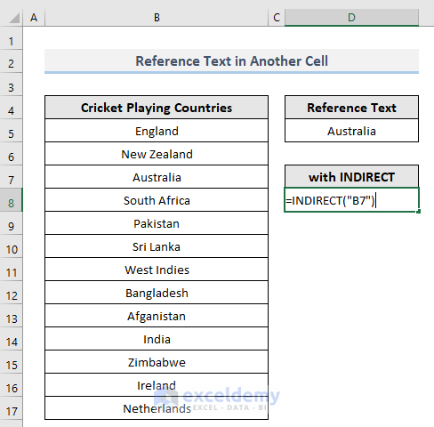
We will take Cell B7 and reference the text, Australia, from it in another cell D8 with the INDIRECT function.
Steps:
- In cell D8, write an equal sign (=), the function name, INDIRECT, and pass the cell reference number that you want to cite the text from inside double quotes (“”).
The formula becomes:
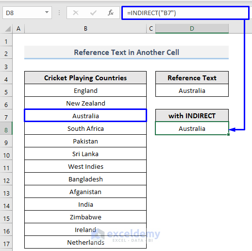
=INDIRECT(“B7”)- Press Enter.
- Look at the following image to check what happened.
Read More: How to Reference a Cell from a Different Worksheet in Excel
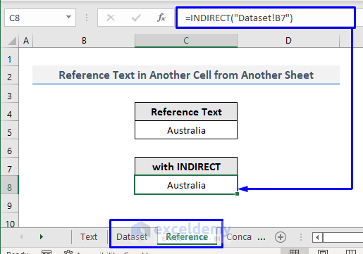
Method 8 – INDIRECT Function to Reference Text from a Cell to Another Cell in Different Worksheet
We have a list in the worksheet named Dataset (shown in Method 2). We will refer to a specific text, Australia from Cell B7, in Cell C5 of the worksheet named Reference (shown in Method 2).
Steps:
- In Cell C8 of the Reference worksheet, write an equal sign (=), the function name, INDIRECT and click on the Dataset.
- Select B7, the cell that you want to cite the text from. Write everything inside the parentheses in double quotes (“”).
The formula in Cell C8 of the Reference worksheet will look like this:
=INDIRECT(“Dataset!B7”)- Press Enter. The text value Australia in Cell B7 of the Dataset sheet is now cited in Cell C5 in the Reference sheet.
Read More: How to Reference Cell in Another Sheet Dynamically in Excel
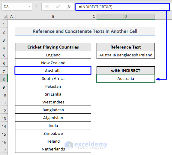
Method 9 – Referencing and Concatenating Texts in Another Cell with the INDIRECT Function
In cell D8, we have to write INDIRECT and pass the reference inside the parentheses inside double quotes (“”). Here is how we passed the reference here:
- We wrote “B” inside double quotes (“”). It means we are passing column B.
- Since we are concatenating here, we put an ampersand symbol (&).
- We then put 7. It means we are passing row number 7.
- This means we are concatenating column B and row 7 inside INDIRECT.
- Cell B7 carries Australia.
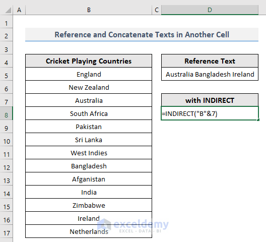
- Press Enter and look at the image below for the result.
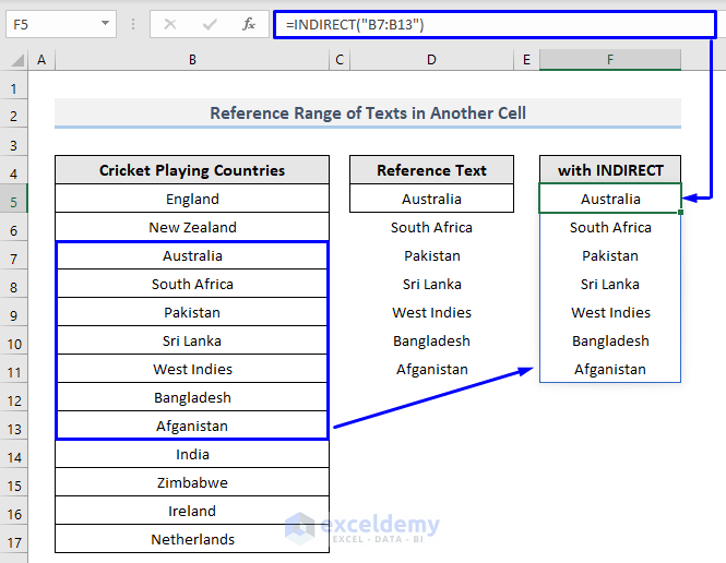
Method 10 – INDIRECT Function to Reference a Range of Texts in Another Cell in Excel
Steps:
- In cell F5, write an equal sign (=), the function name, INDIRECT and pass the range of cell reference numbers that you want to cite the text from inside double quotes (“”).
- Select the first cell from the range that you want to reference the text from and drag to the last cell of the range. For instance, we wanted to reference text value from Australia (in cell B7) to Afganistan (in cell B13) in cell F5, so we selected cell B7 first and dragged to cell B13.
In cell F5, the formula becomes:
=INDIRECT(“B7:B13”)- Press Enter.
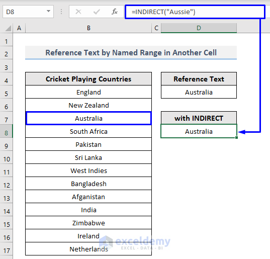
Method 11 – INDIRECT Function to Cite Text in Another Cell with Named Range in Excel
Steps:
- As shown in Method 5, select the cell (B7) that you want to cite the text from and right-click on it.
- Select Define Name…
- Insert any name that you want the cell to have (we named the cell Aussie).
- Click OK.
- In Cell D8, run an INDIRECT function with the defined name (Aussie) inside double quotes (“”) of the parentheses.
The formula will look like this:
=INDIRECT(“Aussie”)- Press Enter.
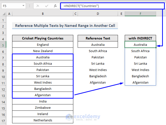
Method 12 – Reference Multiple Texts with Named Range in Another Cell with the INDIRECT Function
Steps:
- As shown in Method 6, select the range of cells that you want to cite and right-click on it. In our case, this is Cell B7 to B13.
- Select Define Name…
- Insert any name that you want the cells to have (we named the cell Countries).
- Click OK.
- In cell D8, run an INDIRECT function with the defined name (Countries) inside double quotes (“”) of the parentheses.
The formula will look like this:
=INDIRECT(“Countries”)- Press Enter.
Method 13 – Reference Text from a Cell to Another Cell with Paste Special in Excel
Steps:
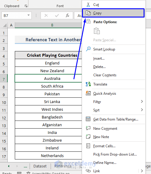
- Select the cell that you want to cite the text form (in our case, it is cell B7).
- Right-click on the cell. A list of options will appear.
- Select Copy from the options or press Ctrl + C from your keyboard to copy the selected cell.
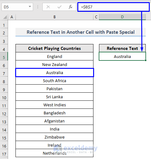
- Go to another cell where you want to reference the text Australia from cell B7. We picked cell D5 to store that.
- Right-click onto the cell (D5) and select Paste Link (N).
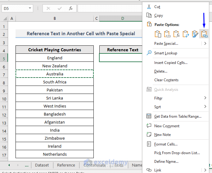
- This will paste the reference value of the copied cell in the target cell. Look at the following image where cell D5 is holding the text value Australia of the cell reference B7 ($B$7 shown in the formula bar).
- Every time you change the value in cell B7, the result cell D5 will automatically be updated according to the text reference.
Read More: Excel VBA Examples with Cell Reference by Row and Column Number
Method 14 – Embed VBA to Reference Text from a Cell to Another Cell in Excel
Steps:
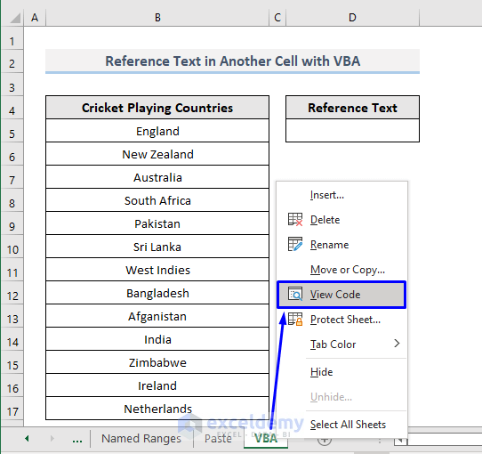
- Right-click on the sheet where you want to implement the referencing.
- Select View Code from the context menu.
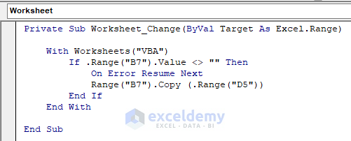
- Copy the following code and paste it into the auto-generated code window:
Private Sub Worksheet_Change(ByVal Target As Excel.Range)
    With Worksheets("VBA")
        If .Range("B7").Value <> "" Then
            On Error Resume Next
            Range("B7").Copy (.Range("D5"))
        End If
    End With
End Sub
Your code is now ready to run.
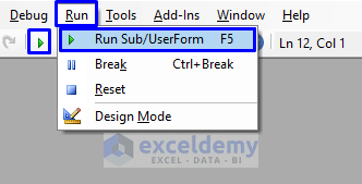
- Press F5 on your keyboard or click on the small Run icon in the sub-menu bar to run the macro.
- After the code execution, look at the gif below to see the result.
Read More: Excel VBA: Cell Reference in Another Sheet
Download Workbook
You can download the free practice Excel workbook from here.
<< Go Back to Cell Reference in Excel | Excel Formulas | Learn Excel
Get FREE Advanced Excel Exercises with Solutions!

Hello,
I have 2 things that i can’t seem to find how to do in excel.
1- How to use custom sort in a sort function?
– Ex: I have a new table with data that aggregates the values of some columns of the raw data table (different sheet), using formulas like, unique, filter, countif, etc.. As i understand it’s not possible to use the sorting methods of the filter button or Data, on the aggregation table because the cells there have formulas. Using the function sort i only have the options of ascending or descending. But one of the columns is Severity and i need to sort by High, then Medium, then Low. How would i do this?
2- How to make the contents of a cell in a column, follow another cell in the same row but on a different column, dinamicaly?
– Ex: In column A i have a list of unique names as the result of index(match(contif)) where the range is in another sheet, in the raw data table. Now in column B i want to write some observations for each name (row) in column A. The raw data sheet will change every time i collect the data. Which means, it will change the order of the names in column A. How to i make sure that the observation that i wrote the first time, remains in the same row as the name?
I appreciate your help.
Thanks, RICARDO SERRÃO for your two amazing queries. Let me help you out in solving your problems.
First, we are going to discuss your first question. The problem you faced is about custom sorting.
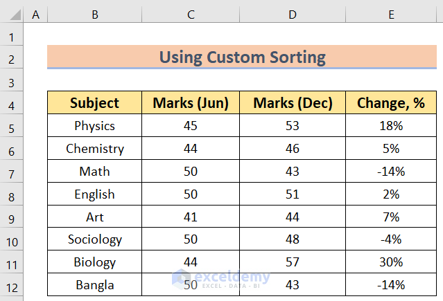
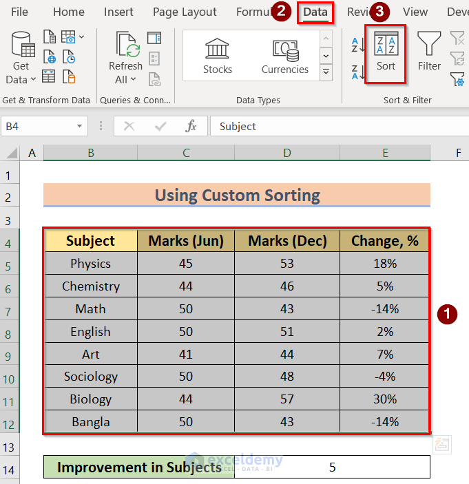
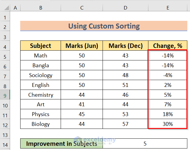
At the very beginning, we arranged a dataset of change in percentage.
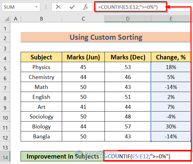
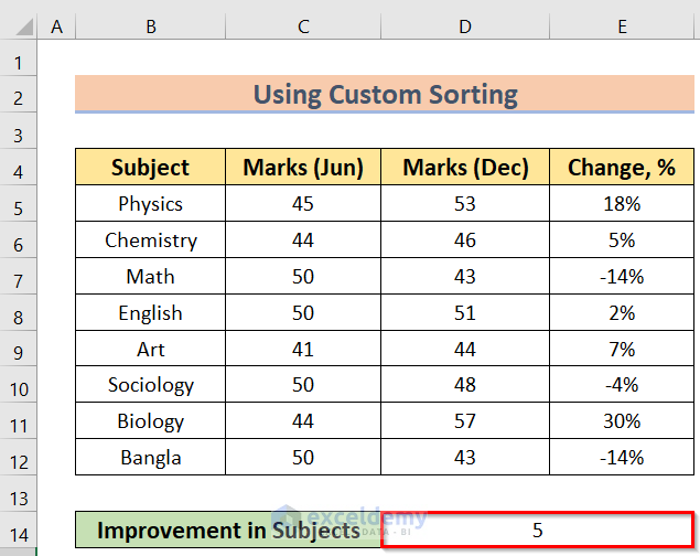
Then, as you wished we have used the COUNTIF function in this dataset.
As a result, we have found the values.
Now, select Dataset> go to Data>Sort options.
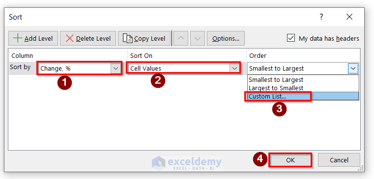
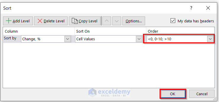
After that, in the Sort window, select Change% in Sort By option, Cell Values in Sort On option, and Custom List in the Order option. Press OK to execute it.
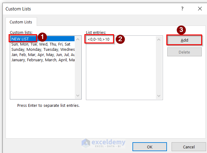
Furthermore, click on the NEW LIST option and write the condition manually in the List Entries area and press Add option.
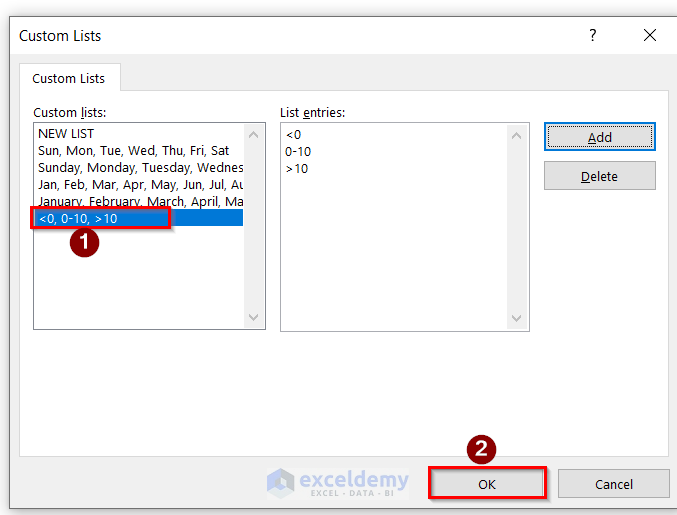
Because of that, you will get the desired condition in the Custom Lists section and press OK.
Afterward, if you can see the desired condition in the Order box then press OK.
Lastly, you will get the result accordingly. As in the condition, you have entered less than zero at first then zero to ten and at last greater than zero that’s why in the Excel section you will get the same order accordingly.
So, that’s the solution to your first query. Now, Let’s go through your second problem.
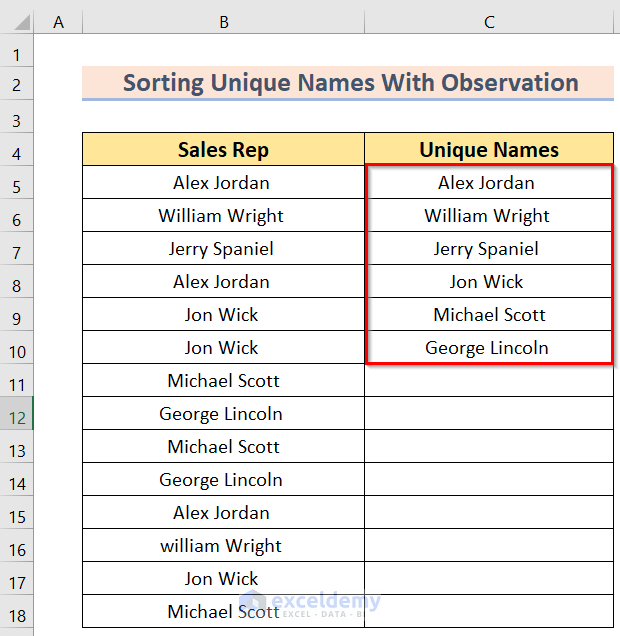
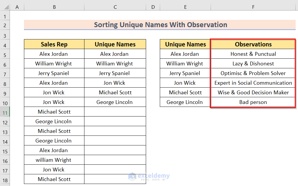
First, by reading your example, at first by using a formula, we created a Uniques Names list.
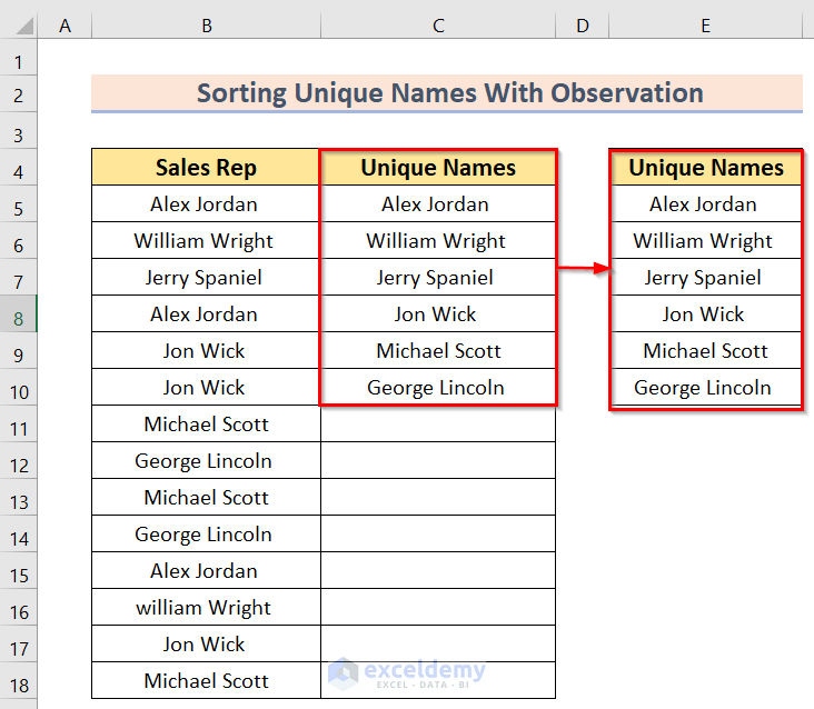
Second, you have to write down the same unique names list in another column. The behind this is, in the array, you can’t use sorting.
Third, then enter the Observations you made next to the new column.
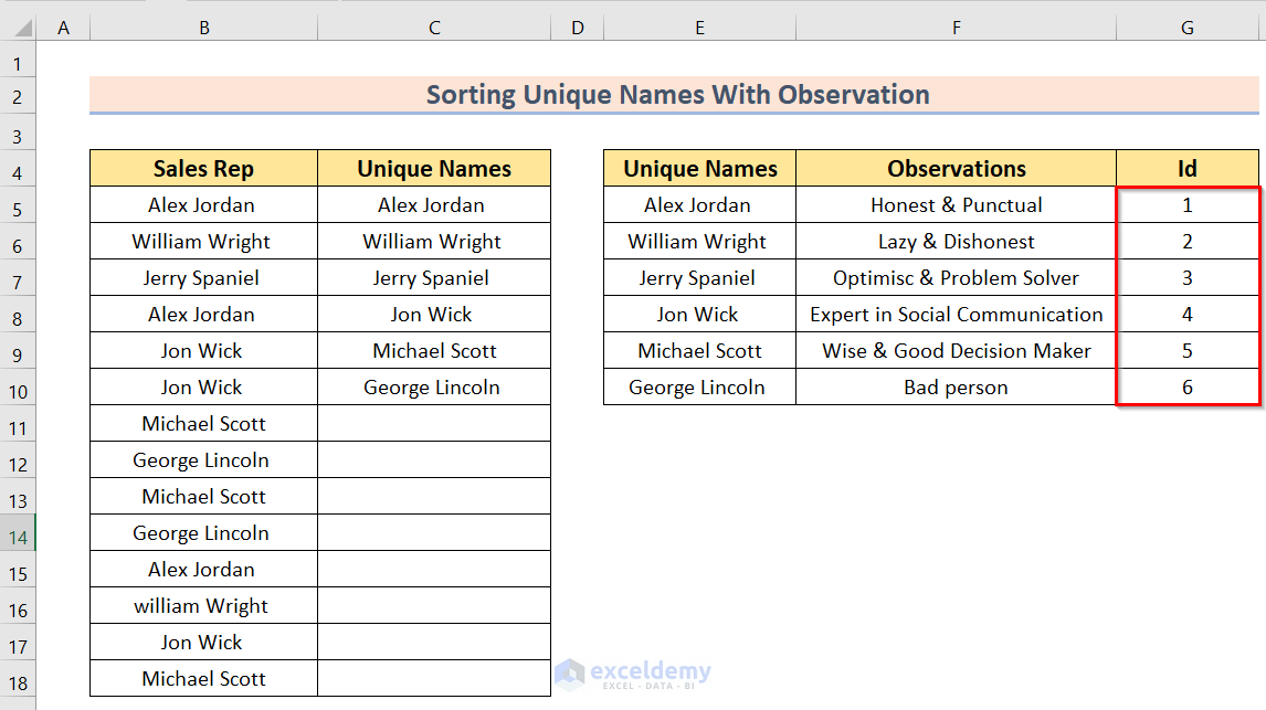
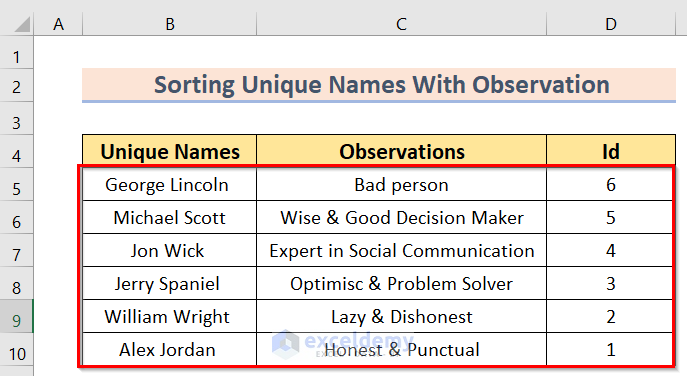
Forth, as we want to sort, so we mark each name with a unique Id number in a new column.
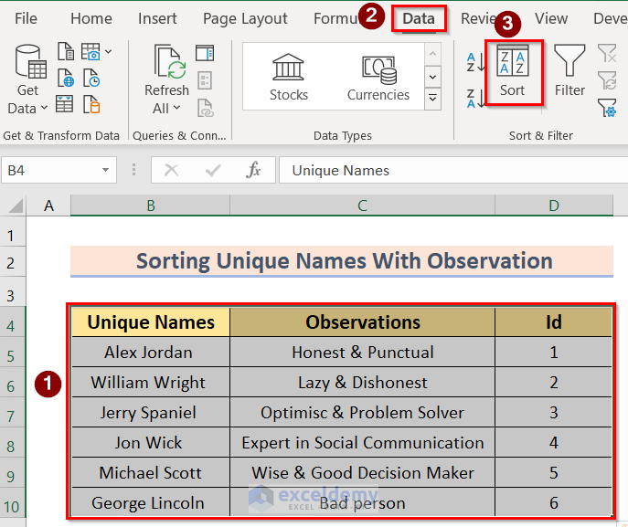
Fifth, go to select the table>Data>Sort options.
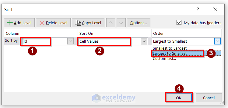
Sixth, select the Id option in the Sort by option, and Cell Values in the Sort On option, click on the Largest to Smallest option in the Order section, and press OK.
Finally, you will get the desired result.
So, this is the solution to your second query.
Therefore, our journey comes to an end. The problems were very fun to solve and I really feel amazed by helping you. Thank you once again. Best of luck.
Hello Zehad,
Im looking for a formula if you would help me find it out. So, if its possible to get your email in order to give you more explanation with screenshots.
Thanks in advance.
Hello Abdallah,
Thank you for reaching out! We’d be happy to help you with your formula. Instead of email, we recommend posting your explanation and screenshots in the ExcelDemy Forum. This way, our community and experts can provide you with a faster and more comprehensive solution.
Looking forward to your post on the forum!
Best regards,
ExcelDemy