How to Keep a Cell Fixed in Excel Formula (4 Easy Ways)

Method 1 – Use the F4 Key in Excel Formula to Keep a Cell Fixed

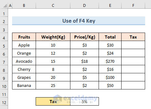
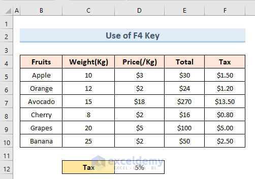
We have a dataset of fruits with their weight, unit price, and total price. Sellers will pay a 5% tax for all kinds of fruits.

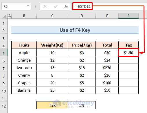
• Select cell F5.
• Insert the following formula:

• Press Enter.
• We get the tax amount for the first fruit item.

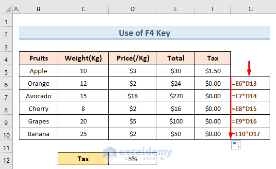
• If we drag the Fill Handle tool, we don’t get any values.
• Look at the subsequent formulas. The cell reference is changing downwards.
• We need to fix the cell value D12 for all the formulas.

• Select cell F5.
• From the formula, select the D12 part and press F4. The formula will look like this:

• Press Enter.
• Drag the Fill Handle to the end of the dataset.

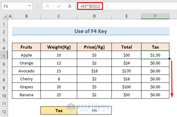
• We get the actual tax amount for all the fruits.

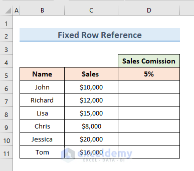
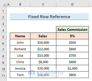
Method 2 – Freeze Only the Row Reference of a Cell

We have the following dataset of six salespeople. Their sales commission rate is 5%. This value is located in Row 5. We will calculate sales commissions for all salespeople, so we’ll fix Row 5.

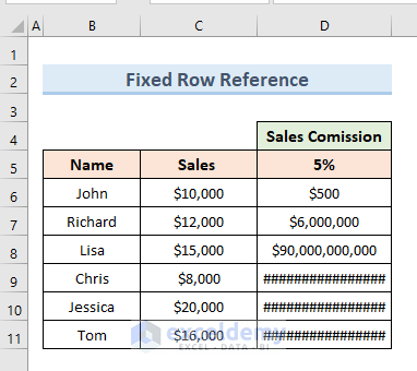
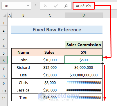
• Insert the following formula in Cell D6.

• We get the amount of sales commission for John.
• Drag down the Fill Handle.

• We get an error because the reference of the value 5% is not fixed in the formula.

• Select the formula of Cell D6.
• Insert a ‘$’ sign before row number 5. Alternatively, press F4 three times.
• Hit Enter.
• Drag down the Fill Handle.

• We get the sales commission value for all the salespeople.

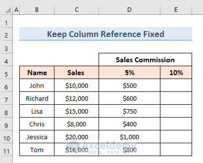
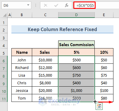
Method 3 – Keep the Column Reference Fixed in an Excel Formula

We will add a new column with a 10% sales commission to our previous dataset.

• Select the cell range (D6:D11).
• Drag the Fill Handle tool horizontally.

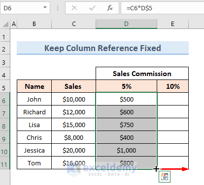
• We get the 10% of the sales commission value of 5%, not of the total sales value. This happens because the column reference wasn’t absolute.

• Select cell D6.
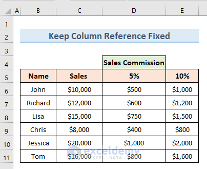
• Insert a ‘$’ sign before column number C to fix the column reference. Alternatively, select the cell reference C6 and press F4 twice.
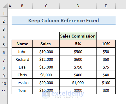
• Drag the fill handle from D6 down, then to the right to fill all cells.

• We get the 10% sales commission for the actual sales value.

Read More: How to Use Cell References in Excel Formula

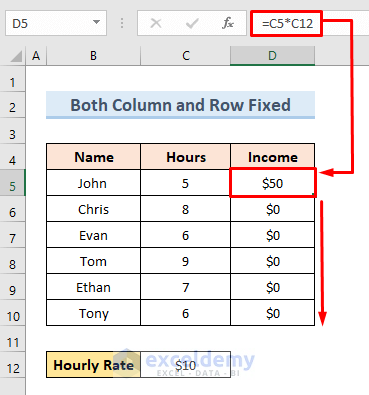
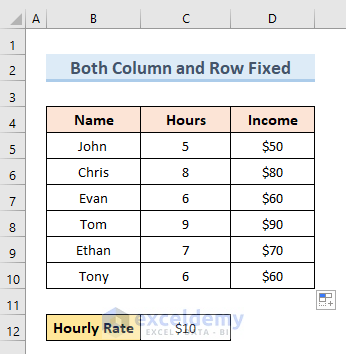
Method 4 – Both Column and Row References of a Cell Fixed

We will use this method in our following dataset of workers to calculate their total income.

• Select cell D5.
• Insert the following formula:

• Press Enter.
• Drag the Fill Handle tool to Cell D10.
• We don’t get the income for all the workers because the cell reference of Cell C12 is not fixed.

• To fix the reference, select the formula of cell D5. Insert dollar signs before C and 12. Alternatively, click on the C12 reference and press F4.
• The formula will look like this:

• Press Enter and drag down the Fill Handle.

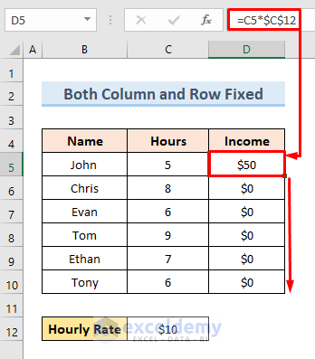
• We get the total income for all the workers.

Download the Practice Workbook

Related Articles

• Relative and Absolute Cell Address in the Spreadsheet
• Difference Between Absolute and Relative Reference in Excel
• Cell Reference in Excel VBA
• Excel VBA: R1C1 Formula with Variable

<< Go Back to Cell Reference in Excel | Excel Formulas | Learn Excel