How to Use Cell Value as Worksheet Name in Formula Reference in Excel

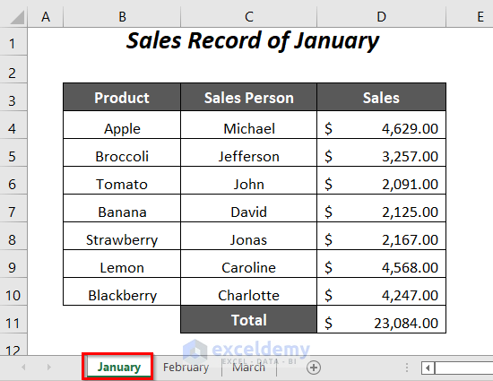
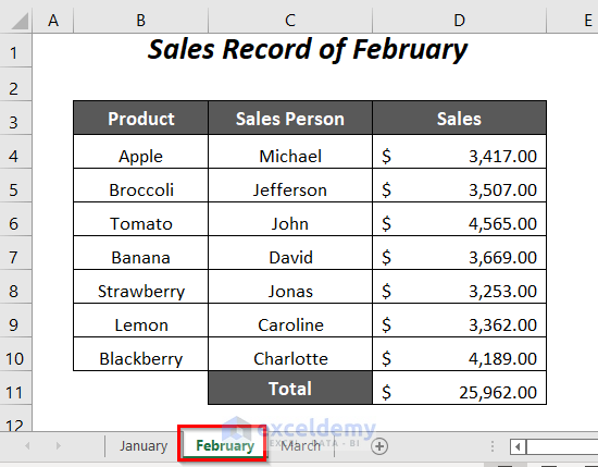
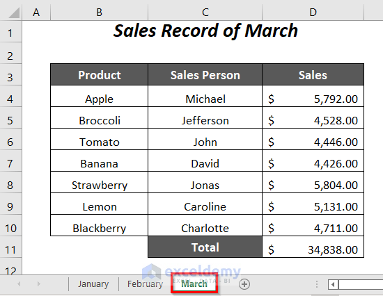
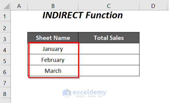
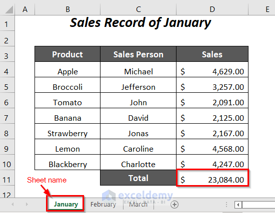
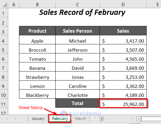
Here, we have 3 worksheets—January, February, and March—containing the sales records of these 3 months for different products. We will use cell values as these worksheet names in a formula as a reference to extract the values in a new sheet.

Method 1 – Using the INDIRECT Function to Use Cell Value as Worksheet Name in a Formula Reference

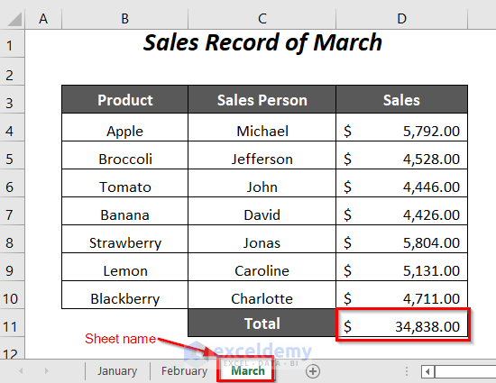
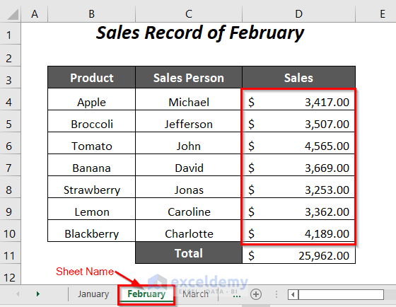
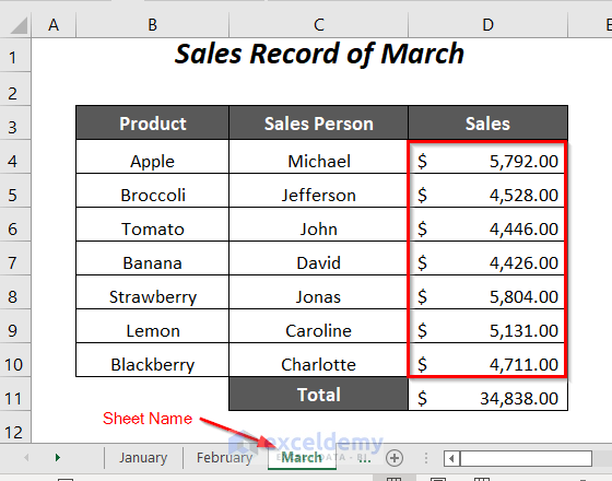
We have the total sales value in cell D11 in each of the three sheets January, February, March.

We put the sheet names as cell values in a new sheet to use as references. Using the INDIRECT function, we will use these values as worksheet names in a formula and it will create a dynamic reference. Let’s get the total sales for each month (available in the three sheets).

Steps:

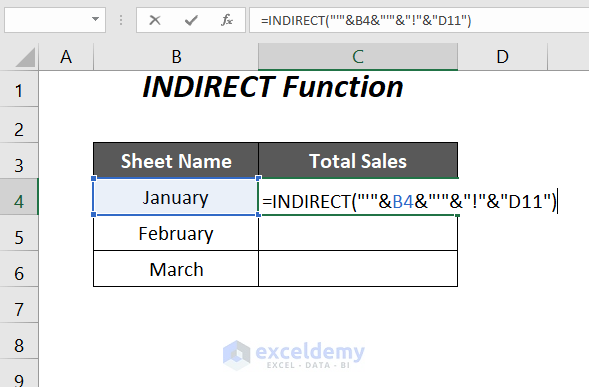
• Insert the following formula in cell C4 of the new sheet:

Here, B4 is the sheet name January and D11 is the cell in that sheet that contains the total sales value.

• Press Enter and drag down the Fill Handle tool.

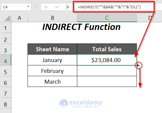
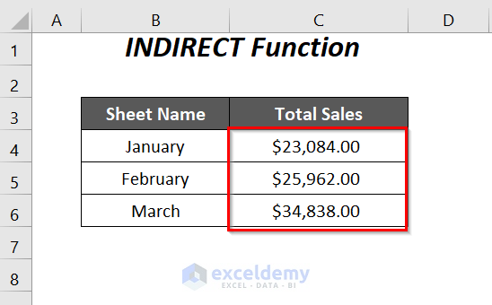
• You will get the total sales values corresponding to the sheet name references in the Sheet Name column.

Read More: How to Find and Replace Cell Reference in Excel Formula

Method 2 – Using INDIRECT and ADDRESS Functions to Use Cell Value as Worksheet Name

In the three sheets January, February, and March we have some records of sales for these months for different products.

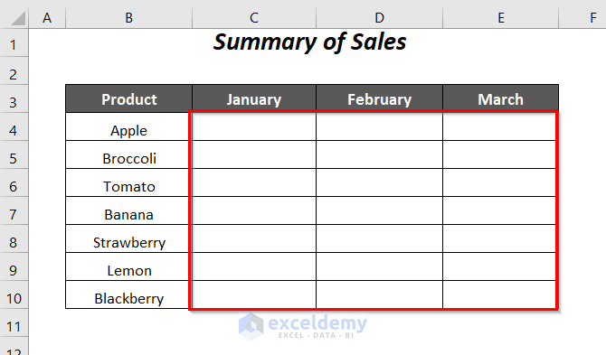
Let’s make a summary table where we will extract the sales values from those sheets and combine them in the January, February, and March columns.

Steps:

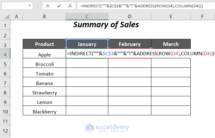
• Insert the following formula in cell C4:

Here, $C$3 is the name of the worksheet.

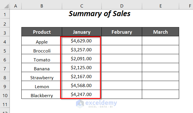
• Press Enter and drag down the Fill Handle Tool.

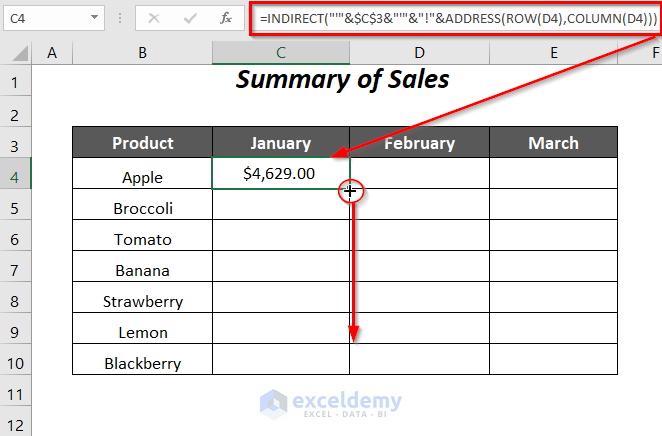
• You will get the sales record from the January sheet in the January column.

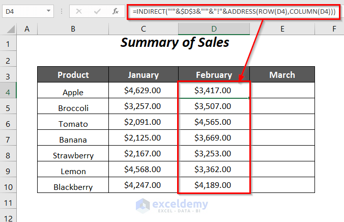
• For the February column, use the following formula in column D.

Here, $D$3 is the name of the worksheet.

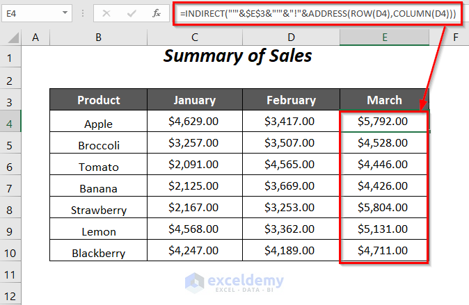
• Similarly, for the sales records of March use the following formula in column E.

Here, $E$3 is the name of the worksheet.

Read More: How to Use OFFSET for Cell Reference in Excel

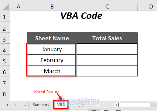
Method 3 – Using VBA Code to Use Cell Value as Worksheet Name in a Formula Reference

Here, we have the total sales value in cell D11 in each of the three sheets January, February, March containing the sales records of January, February, and March.

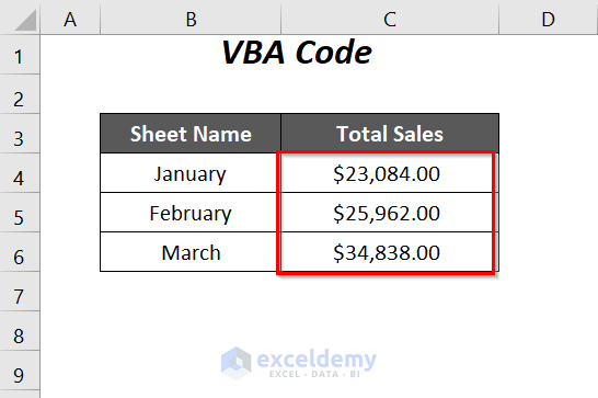
In the Sheet Name column, we have put down the sheet names as cell values. Let’s get the total sales values from these sheets and gather them in the Total Sales column corresponding to their sheet names.

Steps:

• Go to the Developer tab and select Visual Basic.

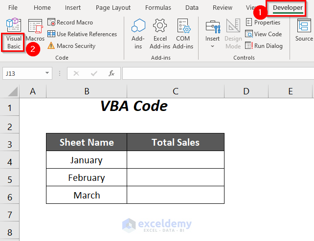
• The Visual Basic Editor will open.
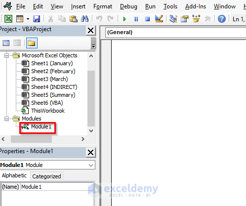
• Go to the Insert tab and select Module.

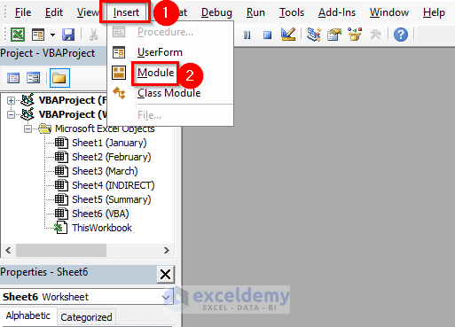
• This creates a blank Module.

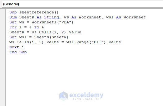
• Insert the following code into it:

Sub sheetreference()
Dim SheetR As String, ws As Worksheet, ws1 As Worksheet
Set ws = Worksheets("VBA")

For i = 4 To 6
SheetR = ws.Cells(i, 2).Value
Set ws1 = Sheets(SheetR)
ws.Cells(i, 3).Value = ws1.Range("D11").Value
Next i

End Sub

Here, we have declared SheetR as String, ws, and ws1 as Worksheet, ws will be assigned to the worksheet VBA where we will have our output. SheetR will store the cell values with sheet names in the VBA sheet. We have assigned the sheets January, February, and March to the variable ws1.

The FOR loop will extract the total sales values from each sheet to the VBA sheet, and here we have declared the range for this loop as 4 to 6 because the values start from Row 4 in the VBA sheet.

• Press F5.
• You will get the total sales values corresponding to the sheet name references in the Sheet Name column.

Read More: How to Reference a Cell from a Different Worksheet in Excel

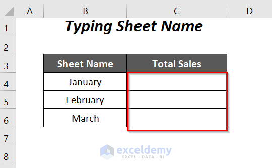
Typing the Worksheet Name for Using Reference in a Formula

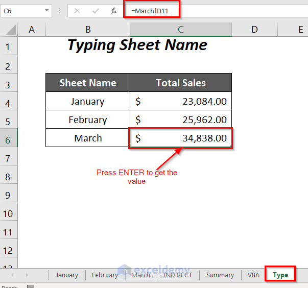
Here, we will extract the total sales values from the sheets January, February, and March, and gather them in the Total Sales column in a new sheet.

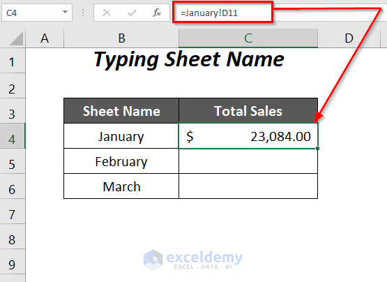
• For the total sales value from January, use the following formula in cell C4:

Here, January is the sheet name and D11 is the total sales value in that sheet.

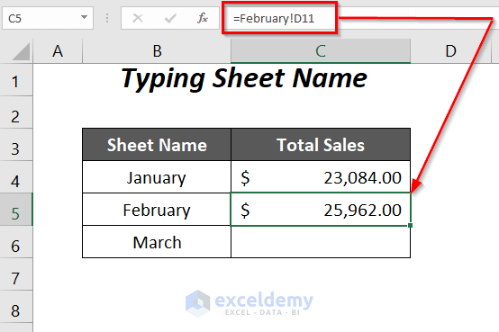
• Similarly, for the sales value of the February month, use the following formula:

Here, February is the sheet name and D11 is the total sales value in that sheet.

If you don’t want to type any formula, you can just select the cell of the March sheet to extract that value in cell C6.

• Type the equals sign (=) in cell C6.
• Click on the March sheet.

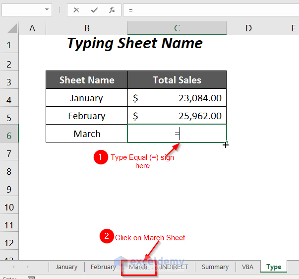
• You will be taken to the March sheet. Select the cell D11 in it.

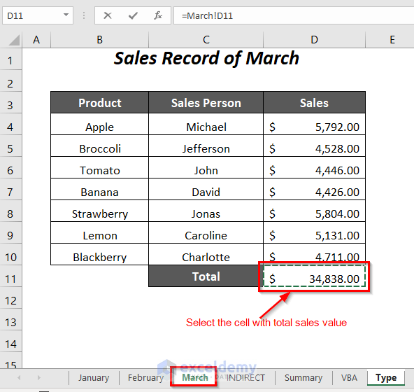
• Press Enter.
• You will get the total sales value for March from that sheet in cell C6 in the Type sheet (the sample sheet we used).

Read More: How to Reference Cell in Another Sheet Dynamically in Excel

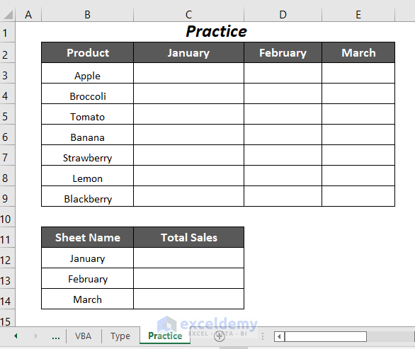
Practice Section

We have provided a Practice section in a sheet named Practice. Download the document below and follow the methods.

Download Workbook

Related Articles

• How to Display Text from Another Cell in Excel 
• How to Reference Text in Another Cell in Excel 
• How to Use Variable Row Number as Cell Reference in Excel
• How to Reference Cell by Row and Column Number in Excel 
• How to Reference a Cell from a Different Worksheet in Excel
• Excel VBA Examples with Cell Reference by Row and Column Number
• Excel VBA: Cell Reference in Another Sheet 

<< Go Back to Cell Reference in Excel | Excel Formulas | Learn Excel