How to Display Text from Another Cell in Excel (4 Suitable Ways)

When using Excel, it is a frequent need for us to display text to a cell from another cell. It is tiring and time-consuming to insert the same values or texts into different cells over and over. In this article, I will show you 4 suitable ways to display text from another cell.

Download Practice Workbook

You can download our practice workbook from here for free!

4 Suitable Ways to Display Text from Another Cell in Excel

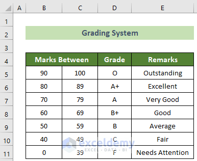
Suppose you have a fixed grading system for an institution.

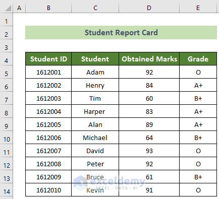
And, you have a dataset of 10 students’ obtained marks and grades per the institution’s grading system.

Now, you want to display text from another cell like displaying a specific student’s grades, formulas, looking up definite values, etc. Read the article carefully below to accomplish these tasks and display text from another cell in Excel.

1. Use Cell Reference to Display Text

Say, you want to display Tim’s grade and remarks upon the grade in other cells. You can use a cell reference to display text from another cell in this regard. Go through the steps below to achieve this.

1.1 From Same Worksheet

📌 Steps:

• Tim’s grade is in cell E7 of the active worksheet.
• So, click on cell G5 and insert the following formula.

• Afterward, hit the Enter button.

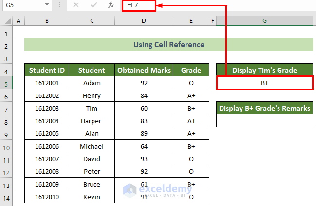
As a result, you will get the grade of Tim in the G5 cell as per your desire.

1.2 From Different Worksheets

📌 Steps:

• Now, the remark for Tim’s grade is in cell E8 of the Grading System worksheet.
• So, click on cell G8 and insert the following formula.

• Subsequently, press the Enter button.

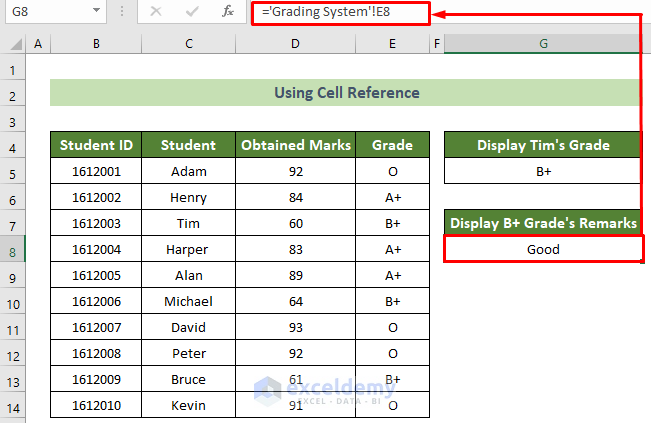
Thus, you will get the remark for Tim’s grade in your desired cell.

2. Use Named Range to Display Text from Another Cell

You can also use named ranges for accomplishing the previous task. Say, you want to display Tim’s grade in cell G5. Follow the steps below to achieve this by using named ranges.

📌 Steps:

• First, you need to create a named range for Tim’s grade.
• To do this, click on cell E7 >> go to the Formulas Tab >> Defined Names group >> Define Name option.

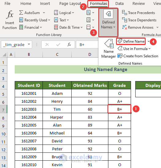
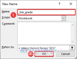
• As a result, the New Name window will appear.
• Following, write _tim_grade in the Name: text box and click on the OK button.

• Afterward, click on cell G5 and insert the formula below.

• Subsequently, press the Enter button.

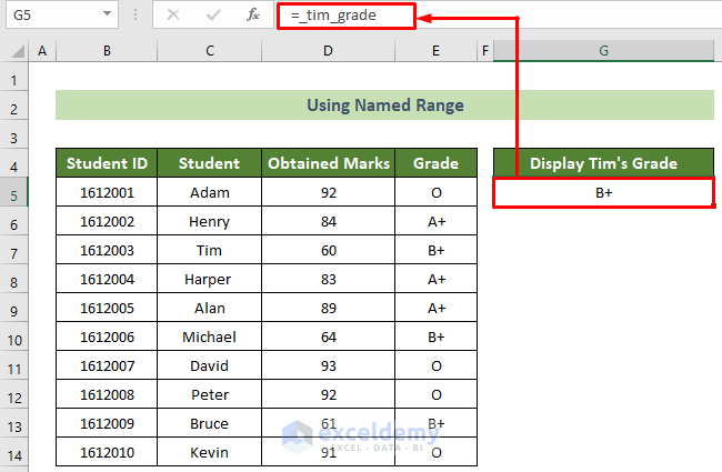
Thus, you will get Tim’s grade displayed in the required cell.

3. Display Formula Text from Another Cell’s Formula

Now, sometimes it might happen that you need the formula of a cell in text. Suppose, you have automated the grades of students according to their obtained marks. Now, you want to display the formula in another cell. Follow the steps below to do this.

📌 Steps:

• At the very beginning, click on cell B17.
• Subsequently, insert the following formula containing the FORMULATEXT function and press the Enter button.

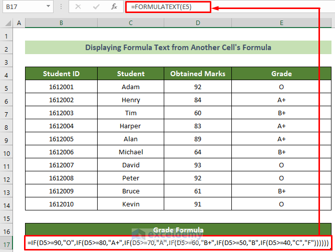
Consequently, the formula for cell E5 will be displayed in cell B17.

4. Use Excel Functions to Display Specific Parts of Text from Another Cell

You can also use the LEFT, MID, or RIGHT functions to display specific parts of a text into another cell.

4.1 Show Left Part of a Text with LEFT Function

Say, you want to display the first 2 letters of cell C10. Follow the steps below to accomplish this.

📌 Steps:

• At the very beginning, click on cell G5.
• Following, insert the following formula and hit the Enter button.

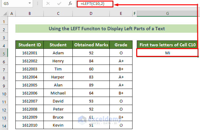
Thus, you will see the first 2 letters shown in cell G5.

4.2 Show Middle Part of a Text with MID Function

Now, say you want to show only the 3 middle letters starting from the 3rd letter of cell C10 on cell G5. Follow the steps below to do this.

📌 Steps:

• First, click on cell G5.
• Subsequently, insert the following formula and hit the Enter button.

As a result, you will get the 3 middle letters starting from the 3rd letter of cell C10 on cell G5.

4.3 Show Right Part of a Text with RIGHT Function

Besides, you can also show the specific right part of a text by following the steps below. Say, you want to show the last two letters of cell C10.

📌 Steps:

• Initially, click on cell G5 and insert the formula below.

• Following, press the Enter button.

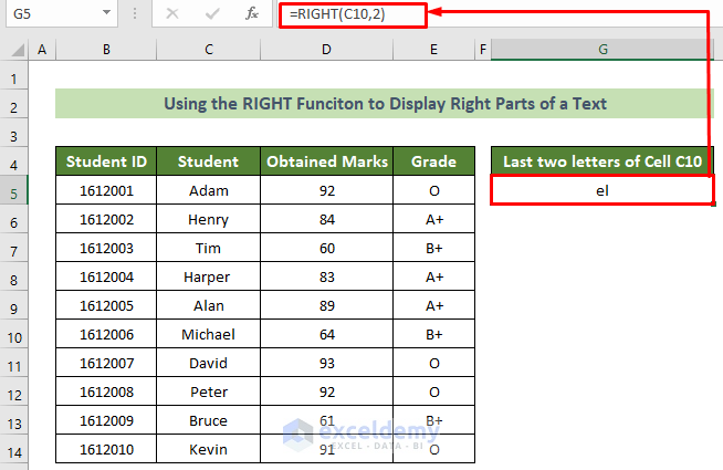
Thus, you will get your desired result.

How to Combine and Display Text from Multiple Cells in Excel

Now, you might need to combine two or more cells and display them in another cell. Say, you want to combine the first student’s name and his obtained mark with a hyphen (-). Go through the following ways to accomplish this.

• Use the Ampersand (&) Operator

You can use the Ampersand (&) operator to achieve your desired result. Follow the steps below to dos this.

📌 Steps:

• At the very beginning, click on cell G5.
• Afterward, insert the following formula.

• Subsequently, press the Enter button.

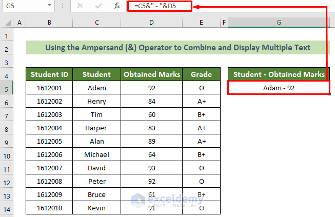
Consequently, you will get your desired result displayed on cell G5.

• Use the CONCATENATE Function

You can also use the CONCATENATE function to accomplish the previous task. Follow the steps below to perform this.

📌 Steps:

• First, click on cell G5.
• Next, insert the following formula.

• Finally, hit the Enter button.

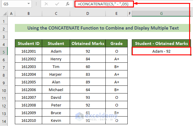
Thus, you will see that you have achieved your desired target.

• Use the TEXTJOIN Function

Moreover, you can use the TEXTJOIN function to combine and display text from other cells. Go through the steps below to do this.

📌 Steps:

• Initially, click on cell G5.
• Subsequently, insert the following formula and hit the Enter button.

Consequently, you will get your desired result.

How to Display Particular Text in Excel Based on Values of Other Cells Using Formula

Apart from all the previous tasks, you can also display particular text based on the values of other cells using formulas.

• Use IF Function

Say, you want to automate the grading system. That is, you want to display grades for every student based on the grading system dataset. Go through the steps below to do this.

📌 Steps:

• Firstly, click on cell E5.
• Afterward, insert the following formula containing the IF function based on the grading system dataset.

• Finally, hit the Enter button.

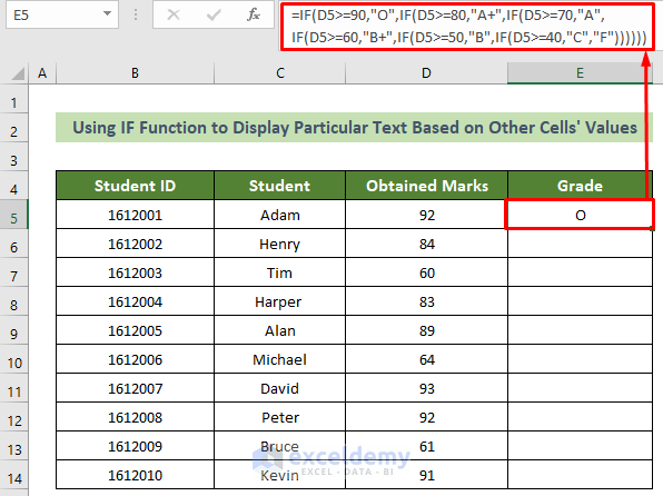
Afterward, you can use the fill handle feature to get the grades for all students based on the grading system dataset.

• Use INDEX-MATCH Formula

Furthermore, you can find a particular student’s grade from the student report card dataset by using the combination of INDEX and MATCH functions. Follow the steps below to do this. Say, you want to find the grade of the student whose name is on cell D16.

📌 Steps:

• First and foremost, click on cell D17.
• Afterward, insert the formula below.

• Subsequently, hit the Enter button.

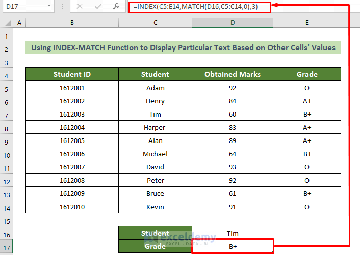
Thus, you will find Tim’s grade from the report card dataset.

Conclusion

So, in this article, I have shown you 4 suitable ways to display text from another cell in Excel.  I suggest you read the full article carefully and practice accordingly. I hope you find this article helpful and informative. You are very welcome to comment here if you have any further questions or recommendations.

And, visit ExcelDemy to learn about many more Excel problem solutions, tips, and tricks. Thank you!