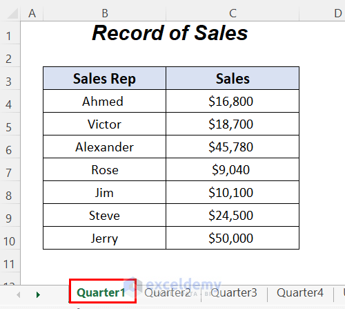
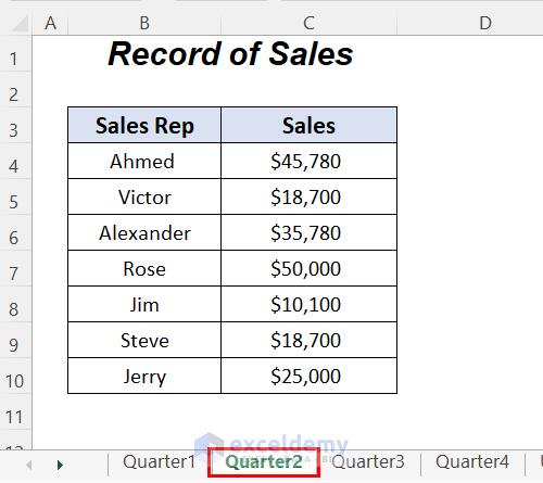
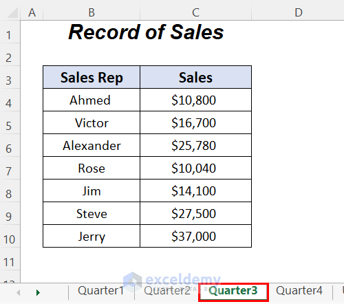
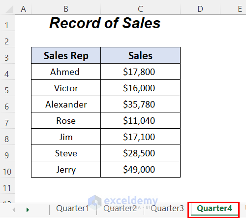
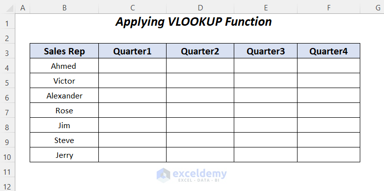
How to Use the Sheet Name in a Dynamic Formula in Excel

There are 4 datasets containing information about sales representatives and their sales: Quarter 1, Quarter 2, Quarter 3, and Quarter 4.

Method 1 – Applying the INDIRECT, IF, OR Functions to Use the Sheet Name in a Dynamic Formula in Excel

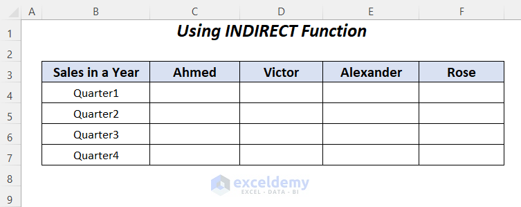
Select C4 cell to keep the Quater1 sales of Ahmed.
Use the formula ( B5 is the sheet from which data will be extracted)
Enter the following formula in C4.

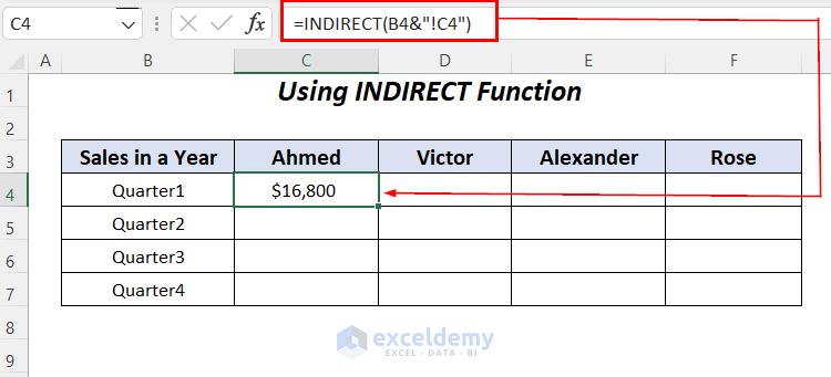
=INDIRECT(B4&"!C4")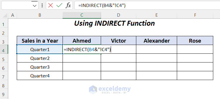

The extracted data from Quater1 is displayed in a new sheet.

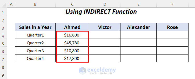
Drag down the Fill Handle to see the result in the rest of the cells.

If the sheet has an empty value, use the IF, and OR functions to avoid the error.

Use the following formula in D4.

=IF(OR(B4="",C4=""),"",INDIRECT(B4&"!C5"))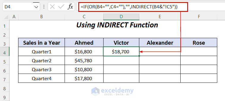

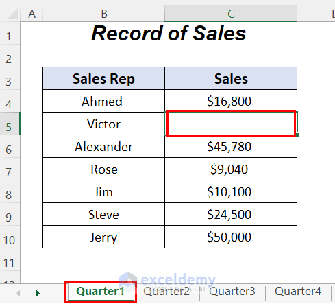
Remove Victor’s Sales from Quater1.

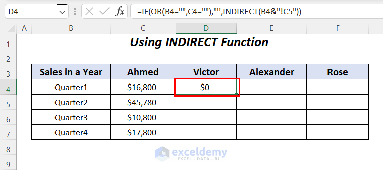
0 is displayed instead of an error because C5 is empty.

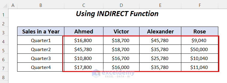
Undo the sales value for Victor and extract data from the 4 Sales Representatives using the AutoFill feature.

Method 2 – Using the VLOOKUP Formula with a Variable Sheet Name in Excel

The dataset was adjusted.

Select the lookup value B4 to extract the Sales data of Ahmed.
Use the INDIRECT function (the sheet name has an absolute row reference).
Enter the following formula in C4.

=VLOOKUP($B4,INDIRECT("'"&C$3&"'!"&"B4:C10"),2,0)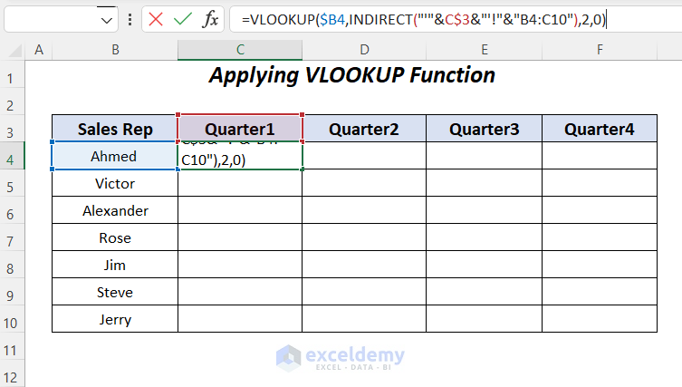

The extracted value for Ahmed is $16,800.

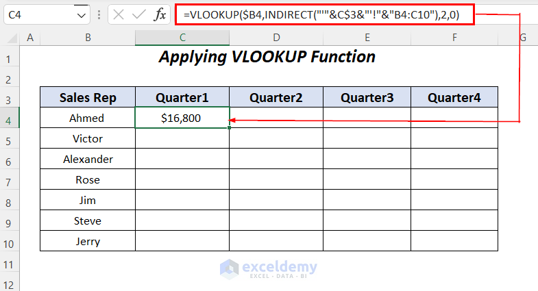
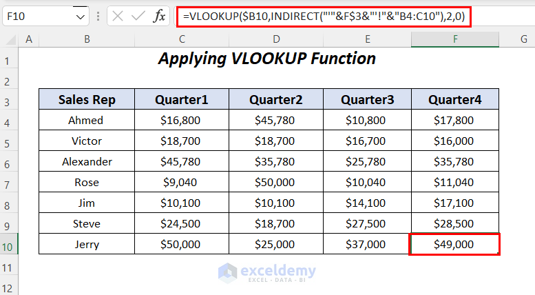
Drag down the Fill Handle to see the result in the rest of the cells.

Method 4 – Applying a Dynamic Formula to Refer to Another Workbook

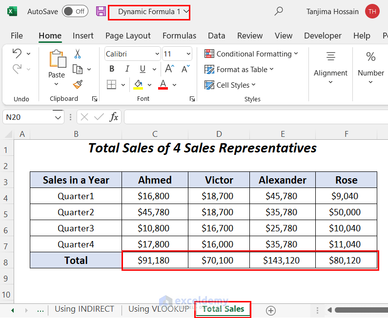
The sample sheet showcases the four sales representatives’ total sales in a year.

Another workbook: Dynamic Formula 2.xlsx was created with a sheet containing the workbook and sheet name. To extract the Total Sales of Ahmed, Victor, Alexander, and Rose :

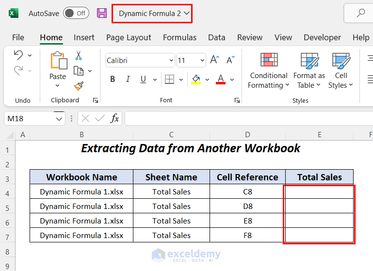
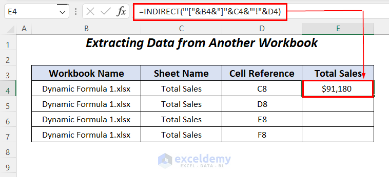
Use the formula in Total Sales, using the INDIRECT function (reference Workbook Name, Sheet Name, and Cell Number).

=INDIRECT("'["&B4&"]"&C4&"'!"&D4)

Keep the referenced workbook open.
To mention the referenced workbook in the formula, use:

=INDIRECT('[Dynamic Formula 1.xlsx]Total Sales'!D4,"")

Here, the first formula will be used.

C8 showcases Ahmed’s data.

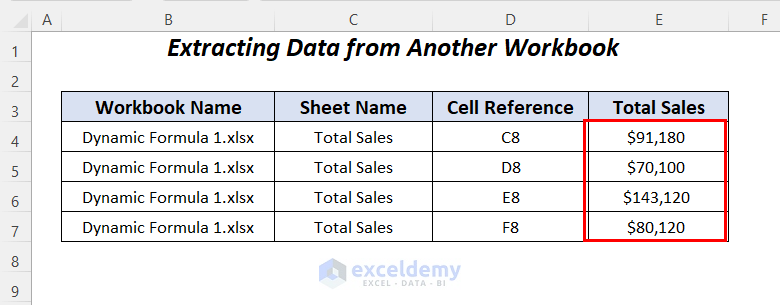
Drag down the Fill Handle to see the result in the rest of the cells.

This is the output.

Practice Section

Practice here.

Download Practice Workbooks

Dynamic Formula 1.xlsx

Dynamic Formula 2.xlsx

<< Go Back to Reference to Another Sheet | Cell Reference in Excel | Excel Formulas | Learn Excel

Get FREE Advanced Excel Exercises with Solutions!

3 Comments

Mark Aug 31, 2022 at 1:38 AM

The workbook is protected and unable to be opened. Therefore, attaching it and allowing for download still does not allow one to “walk” along side your Excel process in pulling this altogether.

Thanks for the article, but please reload a worksheet without the passwords!
- Reply
  Shamima Sep 1, 2022 at 3:45 PM
  
  Hello Mark,
  
  We uploaded the Excel files again, you can check these files also. If you find any difficulty opening the file let us know.
  
  Thanks
- Reply
  Shamima Sep 1, 2022 at 9:47 AM
  
  Hello Mark,
  Hope you are doing well.
  Whenever I try to download this workbook it works fine without a password. To be reassured a couple of my teammates also downloaded this file they also didn’t face any difficulty.
  As I haven’t used any password for this worksheet. I really want to know what caused such issues while you downloaded the file.
  Here, I will show you what it looks like when I download the file again.
  
  After downloading the file Excel shows a warning message. You have to click on Enable Editing.
  
  Later, the downloaded file will be available to use or you can make any changes you want.
  
  N.B. If this solution doesn’t work for you. Kindly sent me the screenshots of the problem.
  
  Thank you.
  
  Regards
  Shamima Sultana