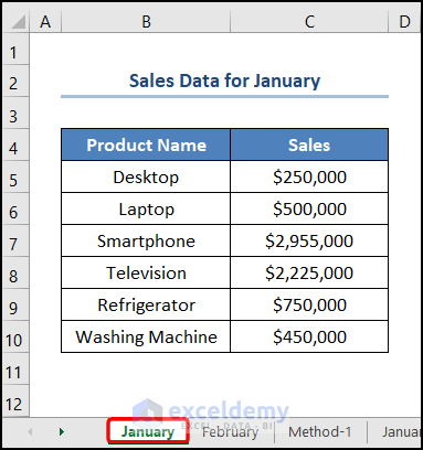
How to Reference Worksheet Name in Formula in Excel

Let’s consider the Sales Data for January in the “January” worksheet, which depicts the “Product Name” and the “Sales” in USD.

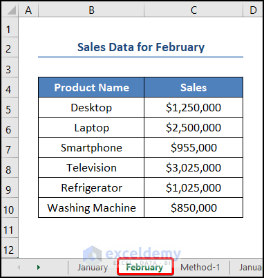
We have the Sales Data for February in the “February” worksheet. We want to obtain the “Total Sales” by pulling in the data from these two worksheets.

Method 1 – Reference a Worksheet Name Without Spaces or Punctuation Characters

Steps:

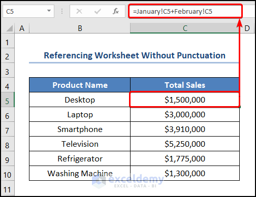
Go to the C5 cell and enter the formula given below.

=January!C5+February!C5

We refer to the worksheet names with exclamation points, and the C5 cell corresponds to the “Desktop Sales” in these two months.

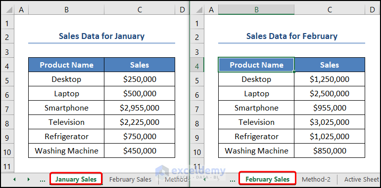
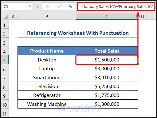
Method 2 – Reference a Worksheet Name with Spaces or Punctuation Characters

We changed the names of the sheets to contain spaces or punctuation.

Steps:

Go to the C5 cell and insert the following:

='January Sales'!C5+'February Sales'!C5

When there are spaces, wrap the sheet name in single quotes (then use the exclamation) to make a reference to that sheet.

Method 3 – Reference a Cell in Another Sheet Dynamically

Steps:

Navigate to the Developer tab and click on Visual Basic.

This opens the Visual Basic Editor in a new window.
Go to the Insert tab and select Module.

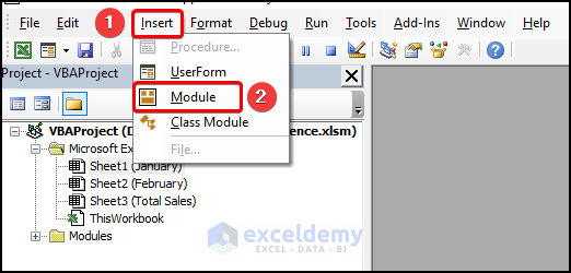
Copy the code from here and paste it into the window as shown below.

Function Active_Work_Sheet_Name()

Dim wbk As Workbook
Set wbk = ActiveWorkbook
Dim result As Variant
Dim j As Variant

j = wbk.Sheets.Count - 1
ReDim result(j, 0)

Dim k As Variant
For k = 0 To j
    result(k, 0) = wbk.Sheets(k + 1).Name
Next k
Active_Work_Sheet_Name = result
    
End Function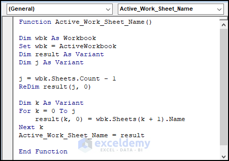

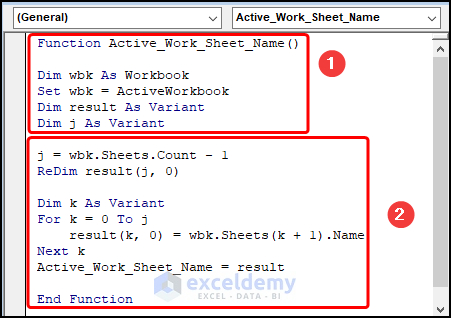
⚡ Code Breakdown:

The subroutine is Active_Work_Sheet_Name().
We define the variables wbk, result, j, and k and assign the data type Workbook and Variant, respectively.

The Count property counts the number of sheets and a For Loop iterates through all the sheets in the workbook.

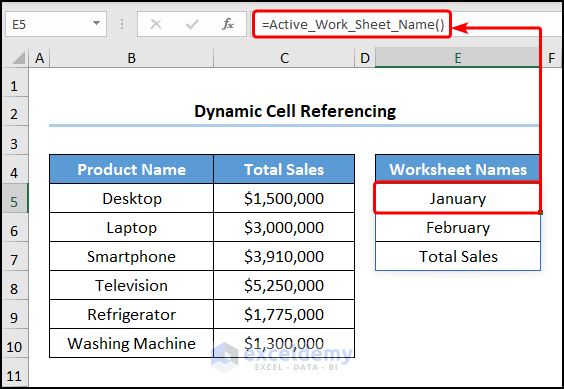
Close the VBA window and enter the function Active_Work_Sheet_Name() to get all the sheet names:

=Active_Work_Sheet_Name()

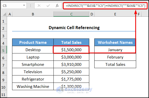
Go to the C5 cell and insert the following into the Formula Bar.

=INDIRECT("'"&E5&"'!C5")+INDIRECT("'"&E6&"'!C5")

The E5 and E6 cells point to the worksheet names January and February, respectively, while the C5 cell refers to their corresponding sales for the product.

Method 4 – Create a Reference to Another Workbook

Steps:

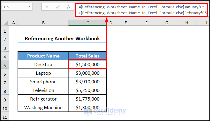
Use the formula below into the C5 cell.

=[Referencing_Worksheet_Name_in_Excel_Formula.xlsx]January!C5+[Referencing_Worksheet_Name_in_Excel_Formula.xlsx]February!C5

“[Referencing_Worksheet_Name_in_Excel_Formula.xlsx]” is the workbook name that contains the “January” worksheet. The workbook needs to be in the same folder as the current workbook.

How to Get the Name of the Active Worksheet in Excel

Steps:

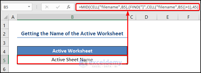
Click on the B5 cell.
Insert the following equation.

=MID(CELL("filename",B5),(FIND("]",CELL("filename",B5))+1),45)

Formula Breakdown:

CELL(“filename”,B5) → returns information about the formatting, and location of the cell contents. Here, the “filename” is the info_type argument which returns the file name and location. Next, the B5 cell is the optional reference argument where the result is returned.
FIND(“]”,CELL(“filename”,B5)) → returns the starting position of one text string within another text string. Here, “]” is the find_text argument while CELL(“filename”,B5) is the within_text argument. Here, the FIND function returns the position of the square brace within the string of text.
- Output → 103
MID(CELL(“filename”,B5),(FIND(“]”,CELL(“filename”,B5))+1),45) → becomes
- MID(CELL(“filename”,B5),(103+1),45) → returns the characters from the middle of a text string, given the starting position and length. Here, the CELL(“filename”,B5) is the text argument, (103+1) is the start_num argument, and 45 is the num_chars argument which represents the maximum number of characters in the worksheet name.
- Output → “Active Sheet Name”

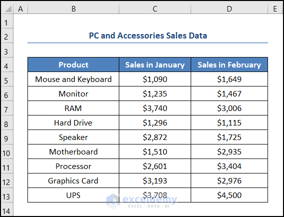
How to Reference Another Sheet Based on Cell Value in Excel

Let’s consider the PC and Accessories Sales Data which shows the “Product” name, the “Sales in January,” and the “Sales in February,” respectively.

Steps:

Go to the Data tab and click on Data Validation then follow the steps shown in the GIF given below.

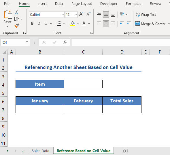
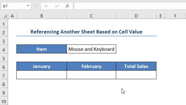
Jump to the B7 cell and use the VLOOKUP function as shown below.

=VLOOKUP(C4,'Sales Data'!B5:D13,2,FALSE)

The C4 cell is the chosen “Item” from the drop-down list.

Formula Breakdown:

VLOOKUP(C4,’Sales Data’!B5:D13,2,FALSE) → looks for a value in the left-most column of a table, and then returns a value in the same row from a column you specify. Here, C4 ( lookup_value argument) is mapped from the ‘Sales Data’!B5:D13 (table_array argument) which is the “Sales Data” worksheet. Next, 2 (col_index_num argument) represents the column number of the lookup value. Lastly, FALSE (range_lookup argument) refers to the Exact match of the lookup value.
- Output → $1090

Refer to the animated GIF shown below.

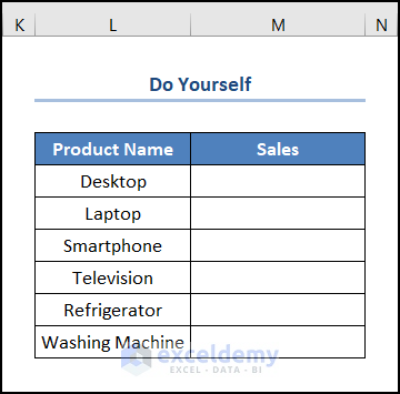
Practice Section

We have provided a Practice section on the right side of each sheet so you can test out these methods.

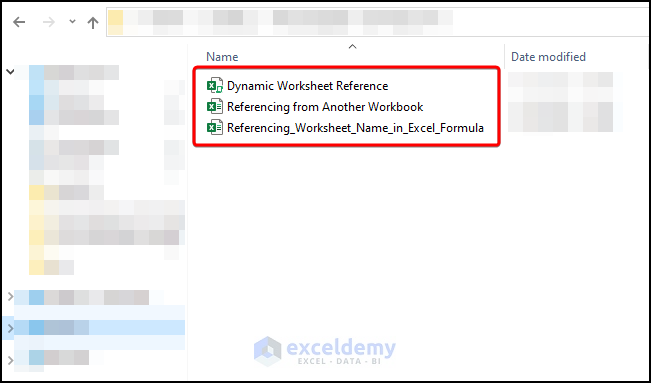
The “Dynamic Worksheet Reference.xlsx” and the “Referencing from Another Workbook.xlsx” files are used in Method 3 and Method 4. In contrast, the “Referencing Worksheet Name in Excel Formula.xlsx” contains the rest of the methods.