The VLOOKUP function is widely used for importing data from a worksheet or workbook. However, due to the function’s argument issue, this function will cause some trouble. Among them, returning a similar value is one. In this article, we are going to demonstrate 2 possible solutions where the VLOOKUP function is returning the same value in Excel. If you are also curious about it, download our practice workbook and follow us.
VLOOKUP Function Is Returning Same Value in Excel: 2 Possible Solutions
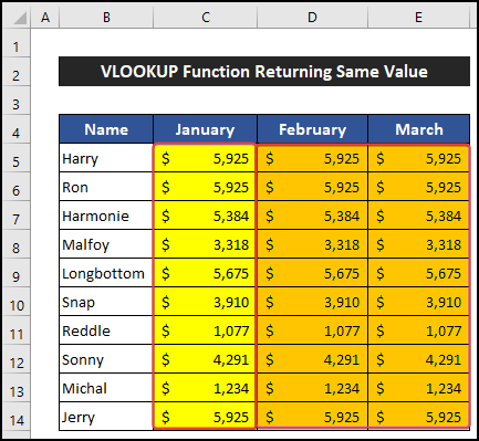
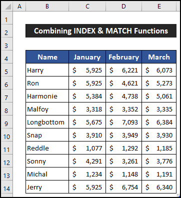
To demonstrate the solutions, we consider a dataset of 10 employees of a company. Their name and the income of the first three months are in the range of cells B5:E14.

Now, if we apply the VLOOKUP function to import the income amount for January, it returns us the correct value. Whereas, when we use the Fill Handle icon to get the value of February and March, it will return the same value as January. The problem you can also notice in the image shown below:
Its solution procedure is described below.
📚 Note:
All the operations of this article are accomplished by using the Microsoft Office 365 application.
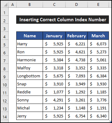
1. Inputting Accurate Column Index Number
Inputting the wrong column index number is one of the common reasons to return the same value for every column. Because when we use the Fill Handle icon to copy the formula of the VLOOKUP function, it does not change the value of the col_index_num. As a result, it provides us with the same result. The steps to fix this problem are given below:
📌 Steps:
- First of all, select cell D5.
- Now, change the col_index_num from 2 to 3.
- Then, press Enter.

- After that, drag the Fill Handle icon to copy the formula upto cell D14.

- You will notice that this time the function will extract the accurate value.
- Similarly, modify the formula for column March.
- Your problem will be resolved.
Thus, we can say that the col_index_num correcting process works effectively, and we are able to solve the issue when the VLOOKUP function returns the same value.
Read More: [Fixed!] Excel VLOOKUP Returning #N/A Error
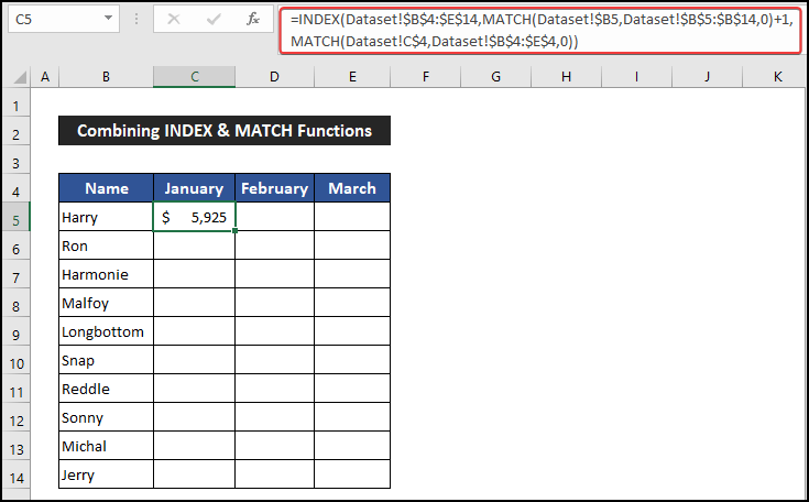
2. Combining INDEX and MATCH Functions
The combination of INDEX and MATCH functions is another way to avoid the problems created by the VLOOKUP function. This combination is very handy, and it can remove all types of errors that we face if we use the VLOOKUP function. The steps of this method are explained below step-by-step:
📌 Steps:
- First, select cell C5.
- Now, write down the following formula in the cell.
- Press Enter.
- Then, drag the Fill Handle icon to copy the formula up to cell E5.
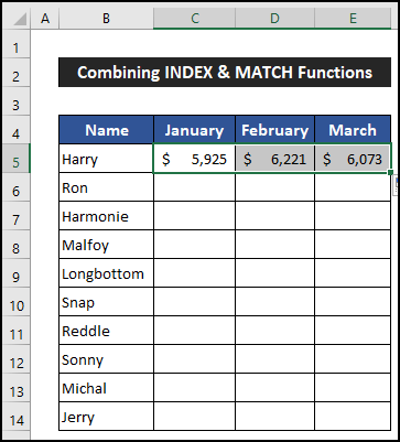
- After that, select the range of cells C5:E5 and drag the Fill Handle icon to copy the formula up to cell E14.

- You will see that all the cells have imported the correct value from the Dataset sheet.
Finally, we can say that our formula works successfully, and we can resolve the problem of getting the same value by the VLOOKUP function by the combination of the INDEX and MATCH functions.
🔎 Breakdown of the Formula
We are breaking down the formula for cell C5.
👉 MATCH(Dataset!$B5,Dataset!$B$5:$B$14,0): The MATCH function will find the position of the value which is in cell B5. Here, the function will return 1.
👉 MATCH(Dataset!C$4,Dataset!$B$4:$E$4,0): Here, the MATCH function will check the relative position of the value which is in cell C5. Here, the function will return 2.
👉 INDEX(Dataset!$B$4:$E$14,MATCH(Dataset!$B5,Dataset!$B$5:$B$14,0)+1,MATCH(Dataset! C$4,Dataset!$B$4:$E$4,0)): Using the value of both MATCH function the INDEX function will extract the income value from the Dataset sheet. For this cell, the value returns $5,925.
Download Practice Workbook
Download this practice workbook for practice while you are reading this article.
Conclusion
That’s the end of this article. I hope that this article will be helpful for you and you will be able to fix the trouble that is the VLOOKUP function returning the same value in Excel. Please share any further queries or recommendations with us in the comments section below if you have any other questions or recommendations.
Keep learning new methods and keep growing!
Related Articles
- Excel VLOOKUP Returning Column Header Instead of Value
- VLOOKUP Is Returning Just Formula Not Value in Excel
- Why VLOOKUP Returns #N/A When Match Exists
- [Fixed] Excel VLOOKUP Returning 0 Instead of Expected Value
- [Fixed!] Excel VLOOKUP Not Returning Correct Value
<< Go Back to Issues with VLOOKUP | Excel VLOOKUP Function | Excel Functions | Learn Excel
Get FREE Advanced Excel Exercises with Solutions!
