The VLOOKUP Function
The VLOOKUP function looks for a given value in a data range and returns the exact match or an approximate match of that value.
- Syntax:
=VLOOKUP(lookup_value,table_array,col_index_num,[range_lookup])- Arguments:
The lookup_value is the given value, table_array is the range in which you to look for a match, col_index_num is the column from which the result is returned, and range_lookup is the match type. The range_lookup is an optional argument here.
VLOOKUP Is Not Returning the Correct Value in Excel: 9 Reasons with Solutions
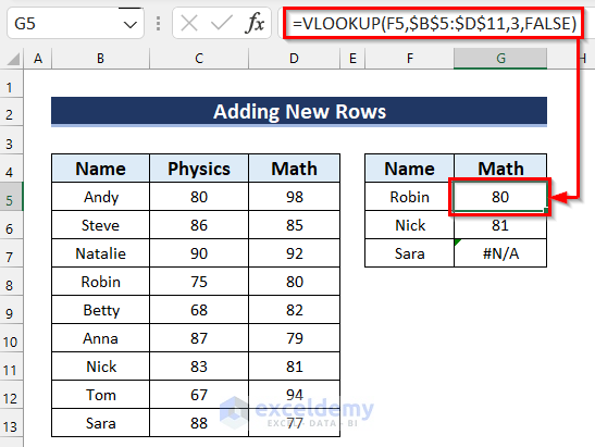
In the following dataset, the VLOOKUP function was used to find the marks in Physics of Natalie.
It is not returning the correct value.
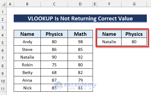
Reason 1 – Not Defining the Match Type
The range_lookup argument was skipped. Excel takes it as TRUE by default, which means an approximate match.

Solution: Define Preferred Match Type Correctly
Steps:
- Select the cell in which you want the result. Here, G5.
- In G5 enter the following formula.
=VLOOKUP(F5,B5:D11,2,FALSE)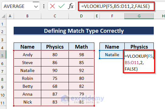
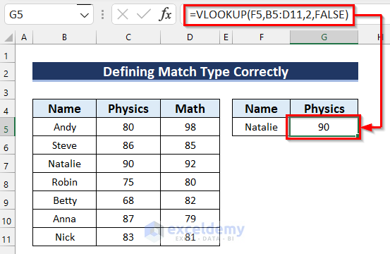
- Press Enter to see the result.
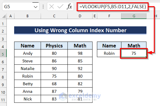
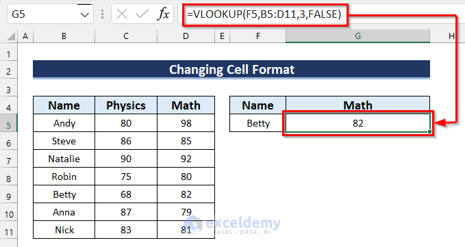
Reason 2 – Using the Wrong Column Index Number
The VLOOKUP function is using the wrong column index number. In the VLOOKUP function, 2 was selected as col_index_num but the marks for math are in column 3.
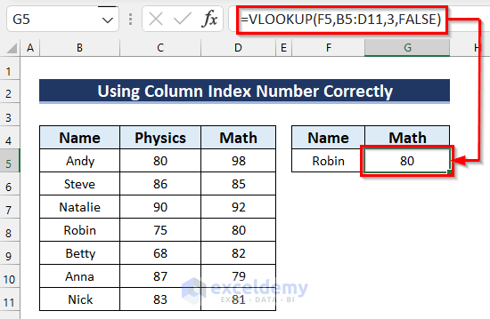
Solution: Use the Column Index Number Correctly
Steps:
- Select the cell in which you want the result. Here, G5.
- In G5 enter the following formula.
=VLOOKUP(F5,B5:D11,3,FALSE)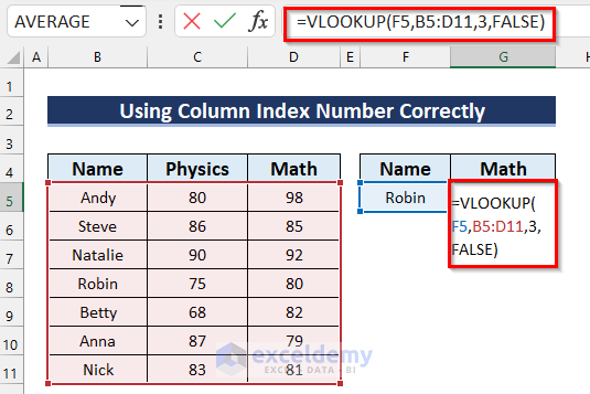
- Press Enter to see the result.
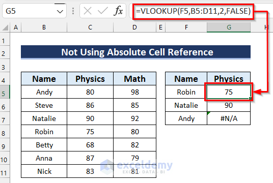
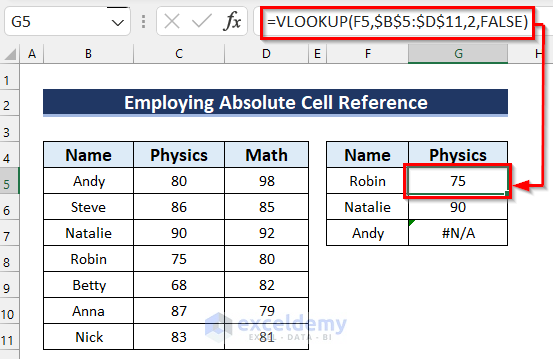
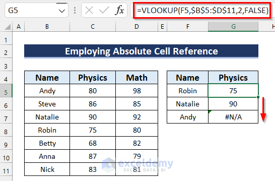
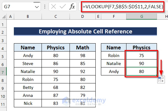
Reason 3 – Not Using an Absolute Cell Reference
The VLOOKUP function is returning the correct value in 2 cases, and in one case it is returning an error. Absolute Cell Reference wasn’t used.
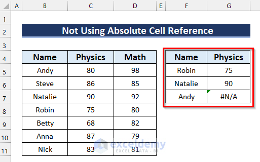
A relative cell reference was used in the VLOOKUP function. It works for the first value but if you drag the Fill Handle to copy the formula, the table_array changes and the function returns a wrong value or an error.
Solution: Apply an Absolute Cell Reference
Steps:
- Select the cell in which you want the result.
- Enter the following formula in that cell.
=VLOOKUP(F5,$B$5:$D$11,2,FALSE)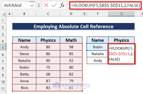
- Press Enter to see the result.
- Drag the Fill Handle down to copy the formula.
This is the output.
Read More: [Fixed] Excel VLOOKUP Returning 0 Instead of Expected Value
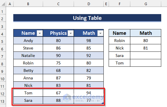
Reason 4 – New Rows Are Added to the Range
The VLOOKUP function is returning wrong values. New rows were added to the range after entering the formula.
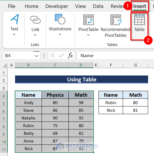
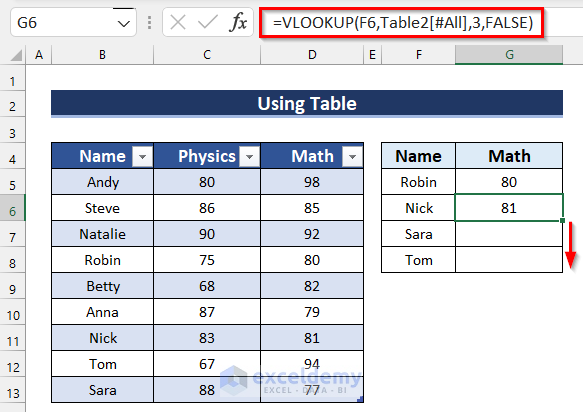
Solution: Use a Table Instead of a Range
Steps:
- Select the range.
- Go to the Insert tab.
- Select Table.
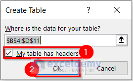
- In the Create Table dialog box, check My table has headers.
- Click OK.
A table will be inserted.
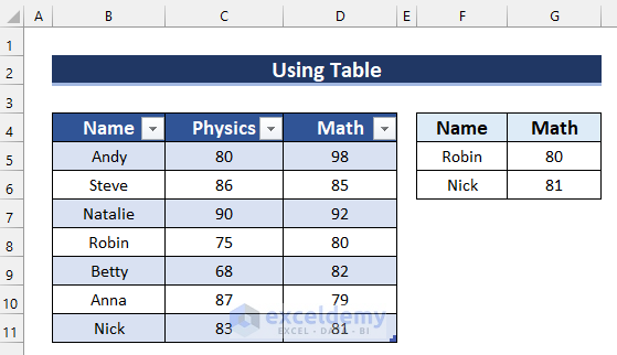
- Select the cell in which you want to find the match. Here, G5.
- In G5, enter the following formula.
=VLOOKUP(F5,Table2[#All],3,FALSE)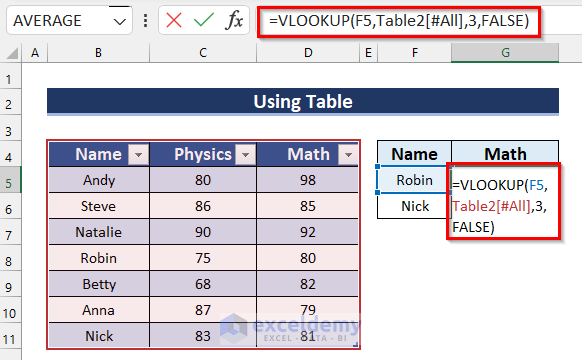
- Press Enter to see the result.
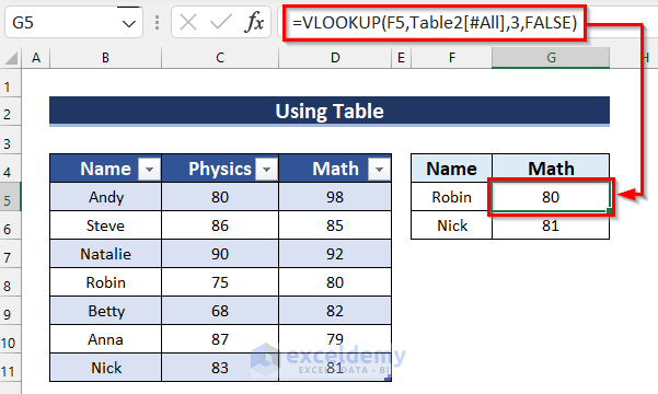
- Drag the Fill Handle down to copy the formula.
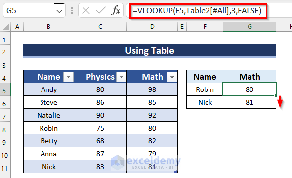
This is the output.
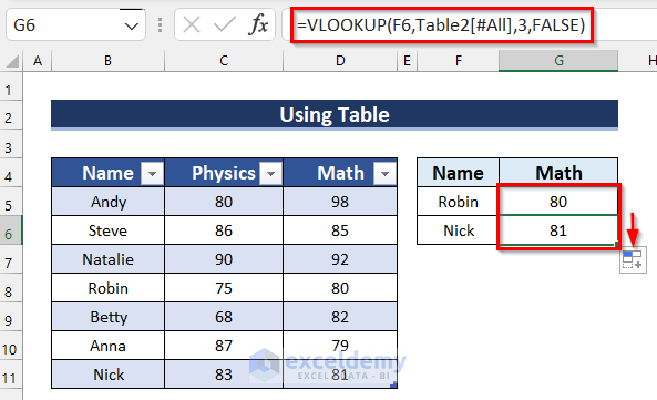
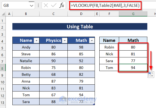
Two rows were added to the table.
- See the correct results for the new values by dragging the Fill Handle.
This is the output.
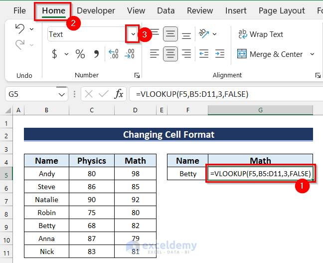
Reason 5 – Selecting Cell Format as Text
The VLOOKUP is not returning the correct value. It returns the formula as it is. Cell format is selected as Text.
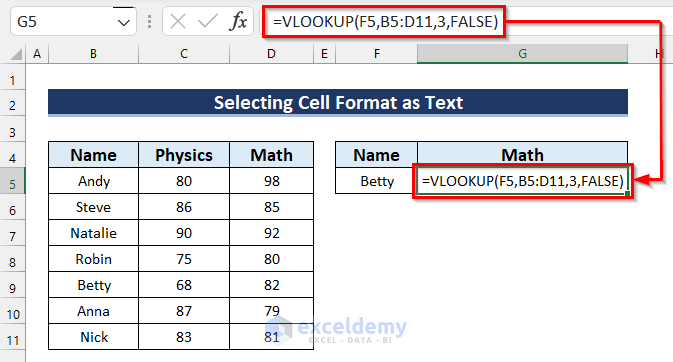
Solution: Change Cell Format & Use the Find and Replace Feature
Steps:
- Select the cell in which the VLOOKUP is not returning the correct value.
- Go to the Home tab.
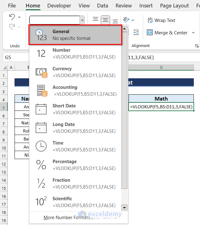
- Select the drop-down option to select cell format.
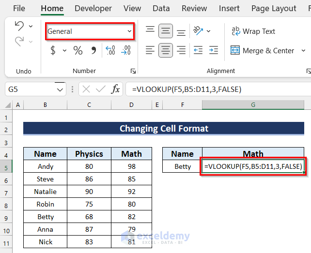
- Select General.
- The cell format is changed to General but the VLOOKUP is still returning a wrong result.
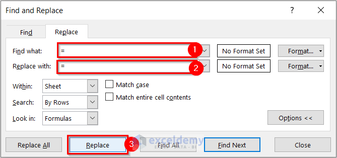
- Press Ctrl + H.
- In the Find and Replace dialog box, enter “=” in Find what.
- Enter “=” in Replace with.
- Click Replace.
This is the output.
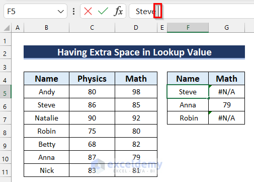
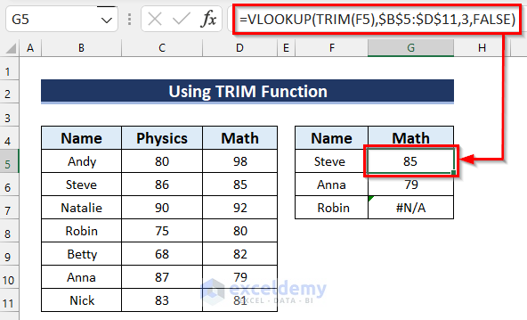
Reason 6 – Having an Extra Space in the Lookup Value
The VLOOKUP formula is correct, but the correct value is not returned.
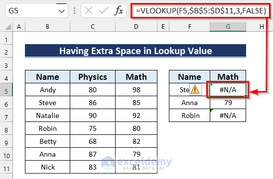
The lookup_value contains an extra space.
Solution: Use the Excel TRIM Function
Steps:
- Select the cell in which the VLOOKUP is returning an error. Here, G5.
- In G5, use the following formula.
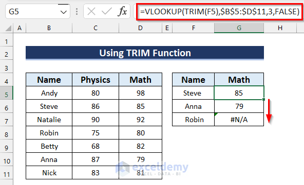
=VLOOKUP(TRIM(F5),$B$5:$D$11,3,FALSE)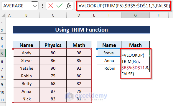
- Press Enter to see the correct result.
Formula Breakdown
- TRIM(F5): removes the extra spaces from the lookup_value.
- VLOOKUP(TRIM(F5),$B$5:$D$11,3,FALSE): TRIM(F5) is the lookup_value, B5:D11 is the table_array, 3 is the col_index_num, and FALSE is the range_lookup. The function will look for an exact match for the lookup_value of column 3 in B5:D11.
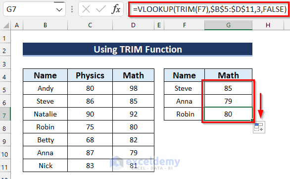
- Drag the Fill Handle down to copy the formula to the other cells.
This is the output.
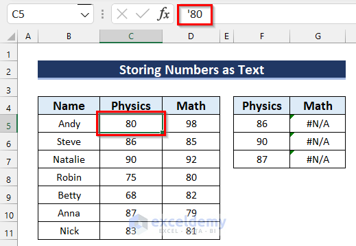
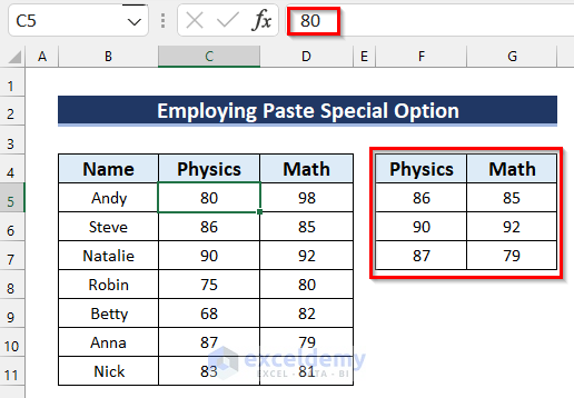
Reason 7 – Storing Numbers as Text
The formula is correct but it is returning an error because numbers are stored as text.
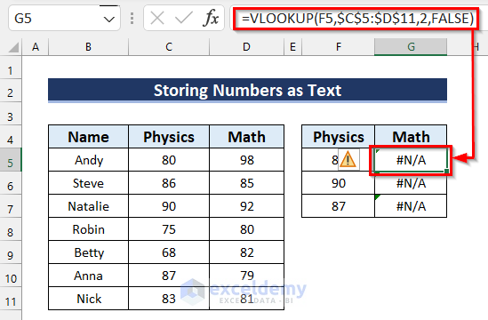
There is an apostrophe before the number.
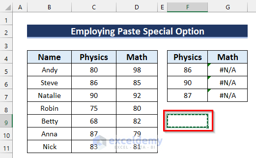
Solution: Using the Paste Special Option
Steps:
- Select a blank cell outside your dataset.
- Press Ctrl + C to copy the cell.
- Select the range in which numbers are stored as Text.
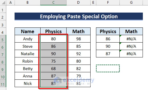
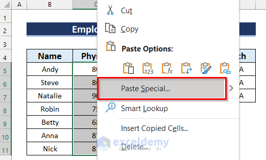
- Right-click the selected cells.
- Select Paste Special.
- In the Paste Special dialog box, select Values in Paste.
- Choose Add in Operation.
- Click OK.
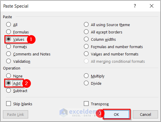
It is returning the correct result.
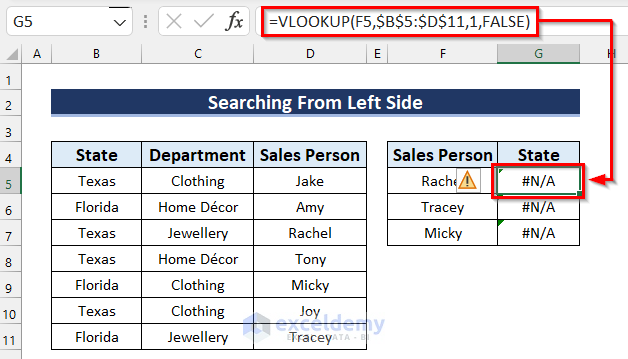
Reason 8 – Searching from the Left Side of the Lookup Value
In the following image the lookup_value is in column 3 and the col_index_num is 1. VLOOKUP can not return the correct value.
Solution: Apply the INDEX and the MATCH Functions
Steps:
- Select the cell in which you want to find the match.
- Enter the following formula in the selected cell.
=INDEX(B5:B11,MATCH(F5,D5:D11,0))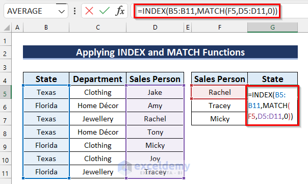
- Press Enter to see the result.
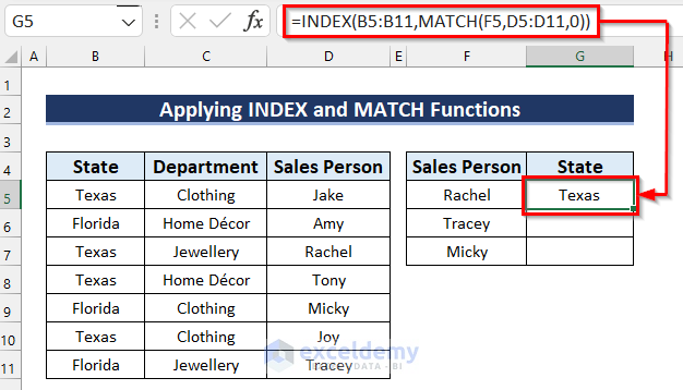
Formula Breakdown
- MATCH(F5,D5:D11,0): finds the exact match of the lookup_value from the lookup_array and returns its relative position in the array.
- INDEX(B5:B11,MATCH(F5,D5:D11,0)): returns the value in B5:B11.
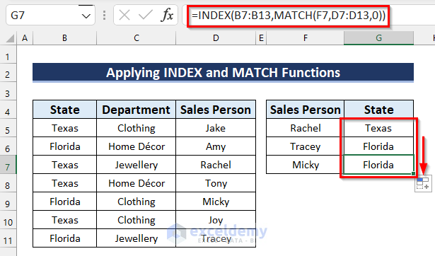
- Drag the Fill Handle down to copy the formula to the other cells.
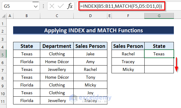
- This is the output.
Read More: [Fixed!] Excel VLOOKUP Returning #N/A Error
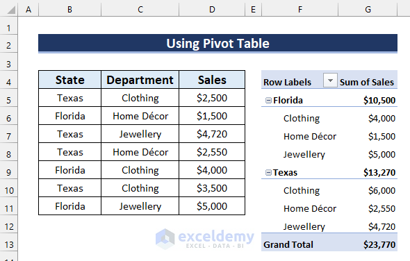
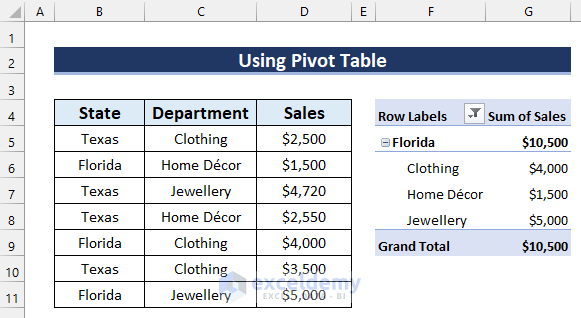
Reason 9 – Table Containing the Same Lookup Value
The table contains the same lookup value multiple times. The VLOOKUP function returns the first value only.
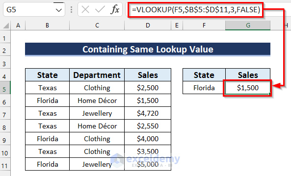
Solution: Use a Pivot Table Instead of VLOOKUP
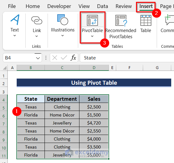
Steps:
- Select the data range.
- Go to the Insert tab.
- Select PivotTable.
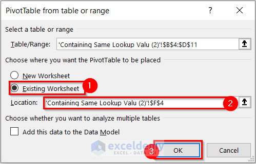
- In the PivotTable from table or range dialog box, select Existing Worksheet.
- Choose a location for the PivotTable.
- Click OK.
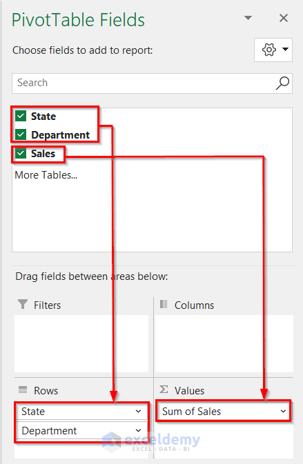
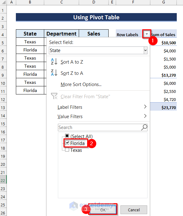
- In the PivotTable Fields Task Pane, select and drag the fields. Here, State and Department into Rows. And, Sales into Values.
The Pivot Table was inserted.
- To filter Florida, click Filter.
- Check Florida.
- Click OK.
This is the output.
Read More: [Fixed!]: VLOOKUP Function Is Returning Same Value in Excel
Download Practice Workbook
Download the practice workbook here.
Related Articles
- Why VLOOKUP Returns #N/A When Match Exists
- VLOOKUP Is Returning Just Formula Not Value in Excel
- Excel VLOOKUP Returning Column Header Instead of Value
<< Go Back to Issues with VLOOKUP | Excel VLOOKUP Function | Excel Functions | Learn Excel
Get FREE Advanced Excel Exercises with Solutions!

Buenas tardes.
Al usar la función BUSCARV en excel, cuando quiero buscar ejemplo 23/03/2023 8:00 al buscar en la matriz solicitada me regresa 23/03/2023 7:00 las 2 tablas están en el mismo libro y tienen formato d/mm/yyyy h:mm
Hello Leonardo,
The issue you’re encountering with VLOOKUP returning the incorrect time (e.g., 8:00 returning as 7:00) may be related to how Excel handles date and time values. Double-check that both columns are formatted exactly the same, not just visually but also in terms of underlying data types (i.e., as date/time values).
Sometimes even slight formatting differences or time zone offsets can cause such issues. You might also try using TEXT functions to standardize the format.
If VLOOKUP is fetching a time that’s off by an hour, consider verifying any regional settings or daylight saving time adjustments.
Regards
ExcelDemy