This is the sample dataset.
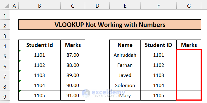
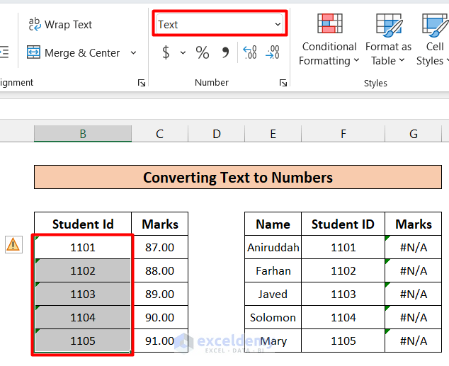
The table on the left showcases Student Ids and their Marks.
The table on the right contains Names, Student IDs and a Marks column.
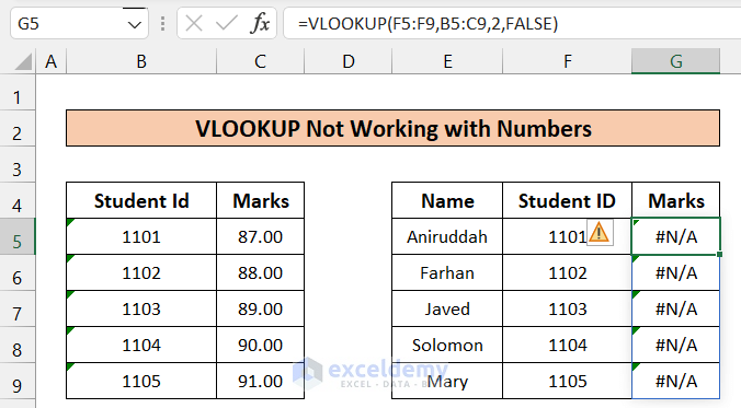
- Enter the following formula in F5.
=VLOOKUP(F5:F9,B5:C9,2,FALSE)the formula looks for a value from F5:F9(Student ID) in the 1st column of B5:C9 and returns the 2nd column value(2) in the array, which is Marks.
An error is displayed.
Solution 1 – Converting Text to Numbers
Steps:
- Select two cells from columns B and F (B5 and F5).
- Enter the following in any cell in the worksheet.
=F5=B5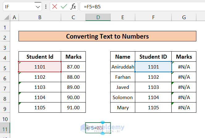
- If the result is TRUE, they have a uniform format. If the result is FALSE, then they have a different format.
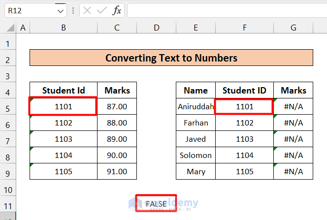
- As the result is FALSE, the formatting needs to be changed.
- Cells in the Student ID: column F are not in Number format. They are in Text format.
To convert the column from text to numbers:
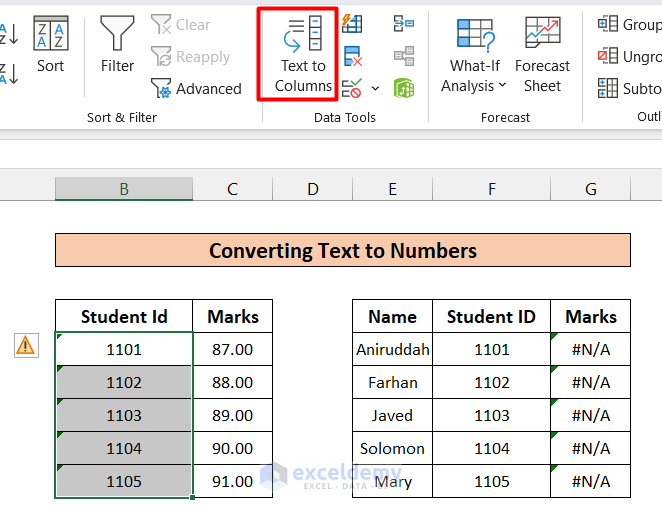
- Select the column (B5:B9).
- In the Data Tab, select Text to Columns.
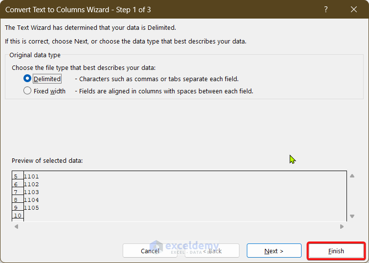
- In the Convert Text to Columns Wizard dialog box, click Finish.
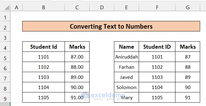
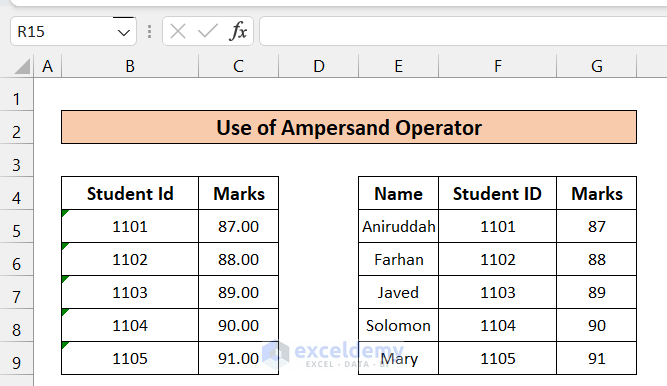
This is the output.
Solution 2 – Use the Ampersand Operator in the VLOOKUP formula
Steps:
- Select G6 cell and enter the following formula.
=VLOOKUP(F5:F9&"",B5:C9,2,FALSE)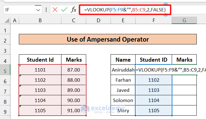
&“” was added after F5:F9 to convert the Text value.
- Press Enter to see the result.
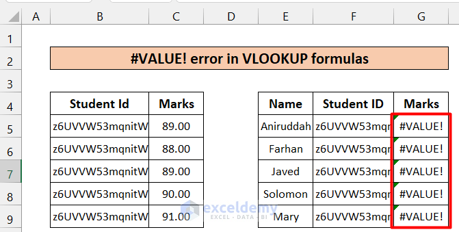
Fixing the #VALUE! Error in a VLOOKUP Formula
If the conditional cells contain more than 255 characters, an error will be displayed.
Steps:
- In G6, enter the following formula.
=INDEX($C$5:$C$9,MATCH(TRUE,INDEX($B$5:$B$9=$F5,0),0))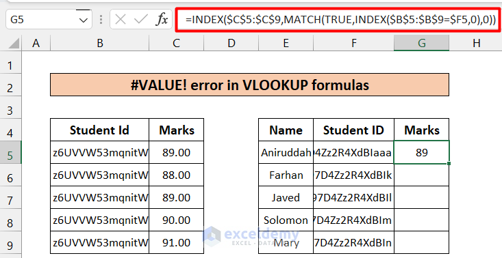
- Drag down the Fill Handle.
This is the output.

Formula Breakdown
- INDEX($B$5:$B$9=$F5,0)
It searches the value in of F5 in (B5:B9) column and returns an array of True (if matched) and False (If not matched).
- MATCH(TRUE,INDEX($B$5:$B$9=$F5,0),0)
The MATCH function returns the row number, which is TRUE in the array, returned by the INDEX function
- INDEX($C$5:$C$9,MATCH(TRUE,INDEX($B$5:$B$9=$F5,0),0))
This returns the value of the cell in the (C5:C9) array, whose row number is equal to the result of the MATCH function.
Things to Remember
- Check the type of data of conditional cells before applying the VLOOKUP function.
Download Practice Workbook
Download the practice workbook to exercise.
Related Articles
- [Fixed!] Excel VLOOKUP Not Working Due to Format
- [Fixed!] VLOOKUP Not Working Between Sheets
- VLOOKUP Not Picking up Table Array in Another Spreadsheet
- [Fixed!] Excel VLOOKUP Drag Down Not Working
<< Go Back to Issues with VLOOKUP | Excel VLOOKUP Function | Excel Functions | Learn Excel
Get FREE Advanced Excel Exercises with Solutions!
