The following VLOOKUP function returned 0 although the matching result is an empty cell.
=VLOOKUP(E5,B5:C12,2,FALSE)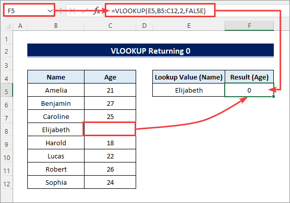
Step 1 – Using the IF Function to Stop the VLOOKUP from Returning 0
- Use the following formula to return blanks:
=IF(VLOOKUP(E5,B5:C12,2,FALSE)="","",VLOOKUP(E5,B5:C12,2,FALSE))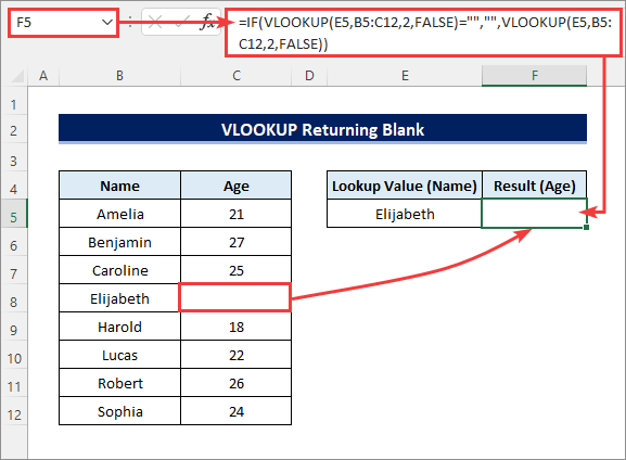
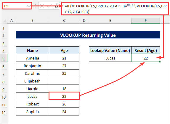
- If you change the lookup_value, the formula will work:
Formula Breakdown: The VLOOKUP function is used twice: as the logical_test argument and as the value_if_false argument of the IF function. The IF function returns blanks if VLOOKUP(E5,B5:C12,2,FALSE)=“” returns TRUE. Otherwise, it returns the output of the VLOOKUP function.
Step 2 – Applying the IFERROR Function to Stop the VLOOKUP Function from Returning Errors
- Use the formula to return blanks if there are errors:
=IFERROR(IF(VLOOKUP(E5,B5:C12,2,FALSE)="","",VLOOKUP(E5,B5:C12,2,FALSE)),"")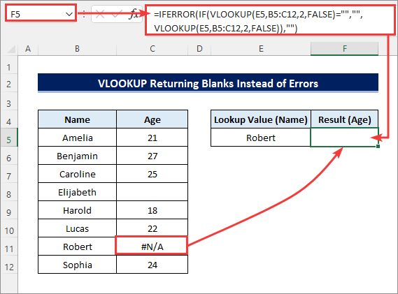
Step 3 – Utilizing the LEN and the ISNUMBER functions
- Use the formula:
=IF(LEN(VLOOKUP(E5,B5:C12,2,FALSE))=0,"",VLOOKUP(E5,B5:C12,2,FALSE))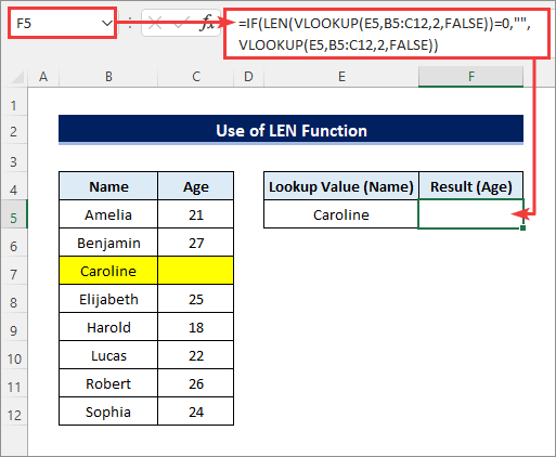
- Alternatively, you can use the ISNUMBER function to return numbers:
=IF(ISNUMBER(VLOOKUP(E5,B5:C12,2,FALSE)),VLOOKUP(E5,B5:C12,2,FALSE),"")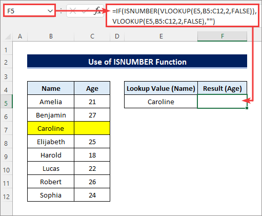
The VLOOKUP Function is Returning Blanks Instead of Values in Excel – Solution
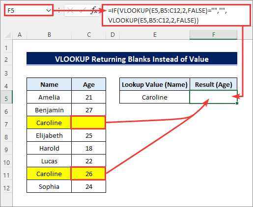
- Use the IF function with the FILTER function:
=IF(FILTER(C5:C12,B5:B12=E5)="","",FILTER(C5:C12,B5:B12=E5))
Formula Breakdown: The FILTER function performs the logical test B5:B12=E5 to filter the matching results for the lookup_value in B5:B12. If the logical_test of the formula FILTER(C5:C12,B5:B12=E5)=”” returns TRUE (empty results), the IF function returns blanks. Otherwise, it returns the output of the FILTER formula.
- Use the TEXTJOIN function to ignore blanks and concatenate other matching results:
=TEXTJOIN(",",TRUE,IF(FILTER(C5:C12,B5:B12=E5)="","",FILTER(C5:C12,B5:B12=E5)))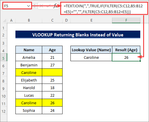
Things to Remember
- Press CTRL + SHIFT + Enter to apply array formulas if you are not using Microsoft 365.
- The VLOOKUP function always considers the first matching result in the lookup_array ignoring all other results.
Download Practice Workbook
Download the practice workbook.
Related Articles
- Why VLOOKUP Returns #N/A When Match Exists
- VLOOKUP Is Returning Just Formula Not Value in Excel
- Excel VLOOKUP Returning Column Header Instead of Value
- [Fixed!] Excel VLOOKUP Returning #N/A Error
- [Fixed!] Excel VLOOKUP Not Returning Correct Value
- [Fixed!]: VLOOKUP Function Is Returning Same Value in Excel
<< Go Back to Issues with VLOOKUP | Excel VLOOKUP Function | Excel Functions | Learn Excel
Get FREE Advanced Excel Exercises with Solutions!
