[Fixed!] Excel VLOOKUP Not Working Due to Format (2 Solutions)

Excel VLOOKUP function is a fantastic function to look up values vertically from a dataset. But, due to different types of errors, the VLOOKUP function does not work properly. The most common problem that happens in this regard is due to format. In this article, I will discuss the Excel VLOOKUP function not working due to format issues and respective solutions.

VLOOKUP Not Working Due to Format in Excel: 2 Solutions

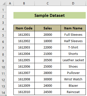
Say, you have a sample dataset of a store with the items’ codes, names, and sales.

Now, you want to use the VLOOKUP function to look up the names of particular items according to their codes or sales. But, due to format errors, you are finding #N/A errors instead of actual results. Now, why is it happening? And what are the solutions? Explore the article below to learn about this thoroughly.

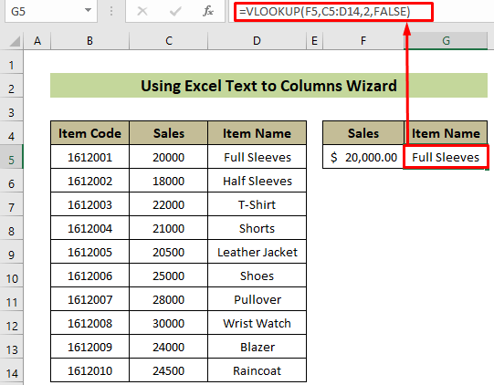
Problem 1: VLOOKUP Not Working Due to Mismatch of Cell Formats

The first factor that can result in this error is the different format of lookup value and lookup column values. Say, you want to find the item name whose sales value is $20,000.

So, you have inserted the VLOOKUP function formula perfectly as follows.

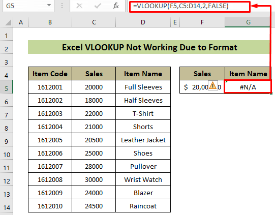
But, the formula is returning a #N/A error. Because the lookup value cell F5 is in Accounting format, but the lookup column values are in Text format.

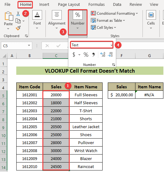
You can check this by selecting cells C5:C14 >> Home tab >> Number group >> Number Format box.

🧲 Solution:

Now, to solve this format issue and to work out the formula properly, go through the steps below.

📌 Steps:

• First and foremost, click on cells C5:C14.
• Following, go to Data tab >> Data Tools group >> Text to Columns tool.

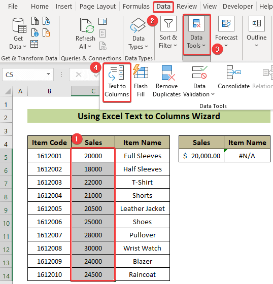
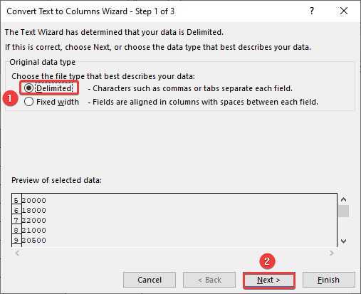
• As a result, the Convert Text to Columns Wizard window will appear.
• Subsequently, choose the Delimited option here and click on the Next button.

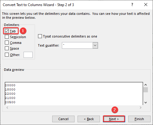
• Afterward, for step 2 of the Convert Text to Columns Wizard, check on the option, Tab from the Delimiters options.
• Subsequently, click on the Next button.

• Afterward, in the third step, choose the option General from the Column data format pane and click on the Finish button.

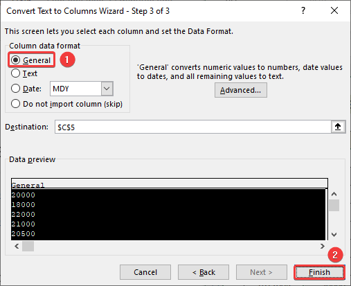
As a result, all the data of C5:C14 cells will be converted from Text to General format. And, the VLOOKUP function would work properly now which would result in the desired item name for the given sales value. And, the output would look like this now.

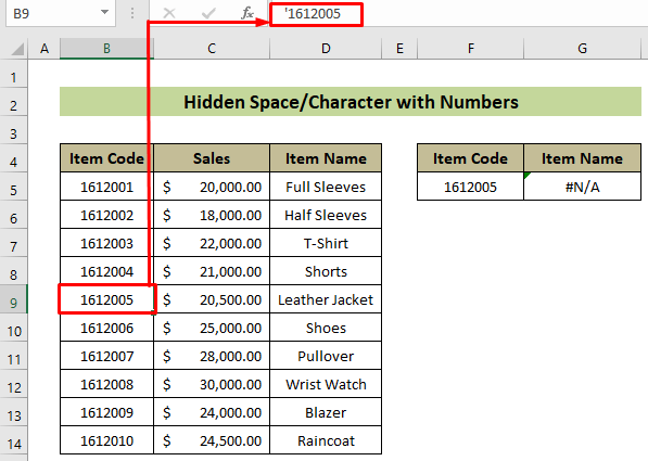
Problem 2: Hidden Space/Characters

Another common problem that is considered to initiate #N/A error in the VLOOKUP function, is hidden spaces or characters. This type of issue mainly happens with numbers.

Say, you want to find item names according to the item codes. Now, you have inserted the formula perfectly as below.

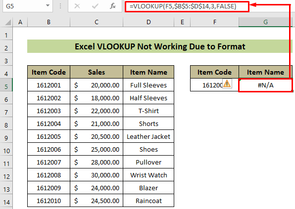
But, the formula is returning a #N/A error for some reason. Now, what is the reason? Let’s find out.

Here, let, you are finding the item name for item code 1612005. This is actually belonging to cell B9. Now, to find the problem if you click on cell B9, you would see there is an apostrophe (‘) just before the actual item code. This apostrophe is not shown in the cell output, but it is converting the code’s format from Number to Text automatically.

So, you have found out that this apostrophe is the problem.

🧲 Solution:

Now, to get rid of this problem and make your VLOOKUP function work, follow the steps below.

📌 Steps:

• First, click on your formula cell (G5 here).
• Afterward, incorporate the TRIM function into cell F5 and cell range B5:D14 in the existing formula. So, the formula would be as follows.

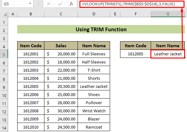
Thus, you will get the VLOOKUP function working perfectly now and you will get your desired result as your issue has been solved.

Download Practice Workbook

You can download our practice workbook from here for free!

Conclusion

So, in this article, I have shown you 2 suitable solutions for the Excel VLOOKUP function not working due to format. I suggest you read the full article carefully and practice accordingly. I hope you find this article helpful and informative. You are welcome to comment here if you have any further questions or recommendations.

Thank you!

Related Articles

• [Solved]: Excel VLOOKUP Not Working with Numbers
• [Fixed!] Excel VLOOKUP Drag Down Not Working
• [Fixed!] VLOOKUP Not Working Between Sheets
• VLOOKUP Not Picking up Table Array in Another Spreadsheet
• [Fixed!] Excel VLOOKUP Function Not Calculating Automatically

<< Go Back to Issues with VLOOKUP | Excel VLOOKUP Function | Excel Functions | Learn Excel