VLOOKUP Not Picking up Table Array in Another Spreadsheet

Solution 1 – Close One if Separate Instances are Open

A worksheet being open in multiple instances is one of the main reasons why the VLOOKUP function does not pick up any table array from another spreadsheet.

Some of the signs that your worksheet is open in another instance are-

Formula references in another open workbook aren’t working.
Copying and pasting from one to the other has fewer options.
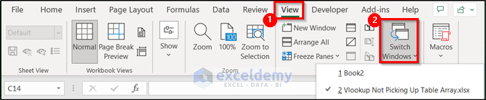
You can check from the Excel ribbon. Open the Switch Windows option from the Windows group of the View, you will find a drop-down with the names of all the workbooks and all the instances that are open.

vlookup not picking up table array in another spreadsheet

Solution:

Close the separate instances of the workbook that are open at the same time.
Note: Even if you haven’t manually opened the workbook separately, it may still happen. Check for the signs above and close the extra workbooks of the same file to make the function pick up from table arrays in another spreadsheet again.

Solution 2 – Check for Correct External References

Another reason that the VLOOKUP function is not picking up the table array in another spreadsheet is the reference for the table array was incorrect in the first place as shown in the sample dataset below.

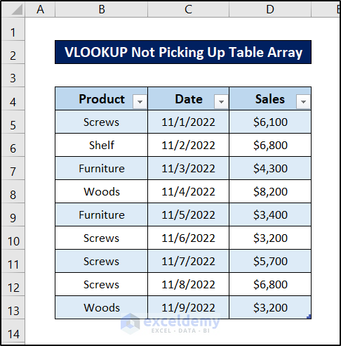
The table starts from cell B4 and ends in cell D13.
If we try to use the VLOOKUP function in the second spreadsheet and we use a wrong reference like the following, an error occurs.

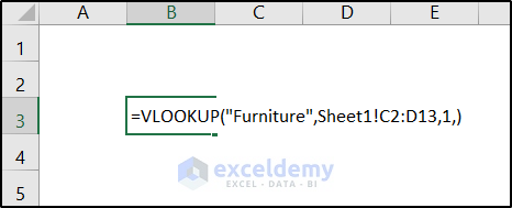
Pressing Enter will give the results as shown below.

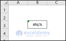
This is because we are looking for the exact match in the wrong reference here. If you use an approximate match, the answer would still be incorrect.

Check for the correct references not only for the cell ranges but also for the sheet names.

Solution 3 – Inspect the File Path for References from Another Workbook

The method to link the formula to an external workbook is to use the file name before the sheet name of where you are taking the reference from, followed by an exclamation mark. Another way to redirect the link is to use the file name before that, as in the following formula.

='/users/user/Google Drive/testfolder/source.xlsx'!cell_name

If any mistake occurs when entering (the one inside the inverted comma), it will search for the wrong direction. This will result in not finding the proper data and the VLOOKUP will not be picking up table array from the spreadsheet of another workbook.
Solution to use the correct formula is to go to the file explorer and double-click the file path on top of the explorer.

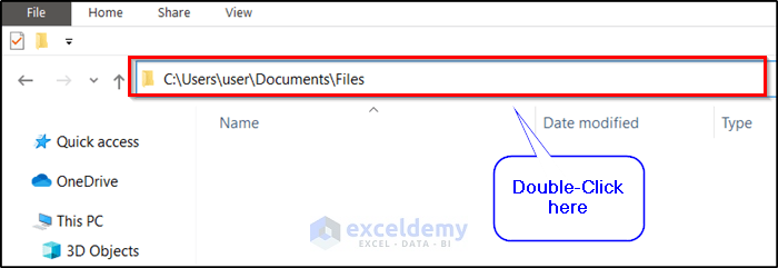
Select the path name, copy it and paste it while entering the file reference to avoid any error.

Solution 4 – Look if the Search Mode is Correct

The fourth argument of the VLOOKUP function is the range_lookup. This is an optional argument that takes a boolean input. It searches for the approximate match if we put a TRUE value in it. Otherwise, it searches for the exact match with a FALSE argument if we initiate it.

Exact match, searches for the exact match for the function. The approximate match will look for the first closest match for the criteria. So, if you do not have the correct search mode as an argument Excel will look for other matches that you might not intend. For example, you want an exact match, but because you entered 1 or TRUE as an argument, Excel will look for the first close match and return the wrong result.

Usually, you put this value in the fourth argument, range_lookup.

Solution 5 – Sort LOOKUP Column

This is a concern if you are looking for an approximate match. What an approximate match does is, it takes the first match from the selected range/array. When you do not have the data sorted within the dataset, the VLOOKUP function will not pick up the correct value from the table array in another spreadsheet or even from the same one.

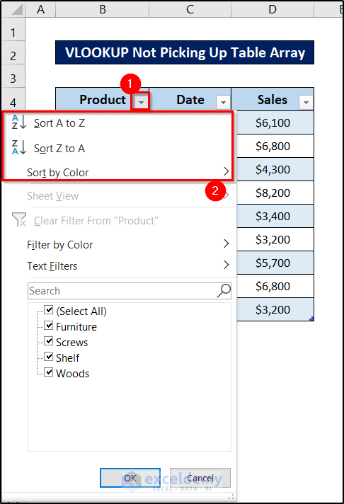
You can sort data manually by selecting and moving cells. If you have the dataset as a table on your spreadsheet, you will have a downward-facing arrow button in the column headers. Click on it to find the sorting options.

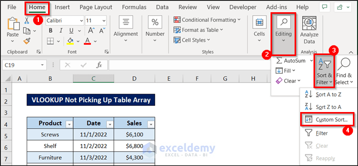
If you want more flexibility, you can find the Custom Sort option through the drop-down menu of the Sort & Filter in the Editing group of the Home tab.

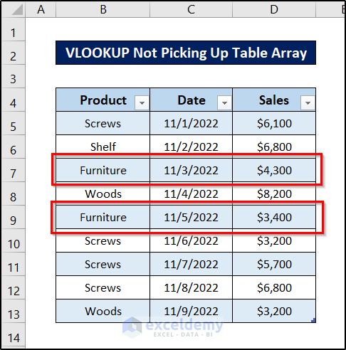
Solution 6 – Check for Duplicates

The VLOOKUP function always looks for the first match no matter the match type. In the case of multiple entries with the same value, the function ignores all of them except the first. So, make sure you don’t have multiple entries with the same argument you are searching for.

Let’s assume we need the following value with the VLOOKUP.

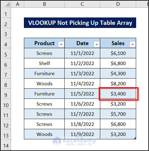
If we apply the VLOOKUP formula in another spreadsheet now from this table array, we will see that it is not picking up the correct value from this table array.

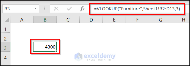
This is because there were two “Furniture” in the table array.

Excel picks up the first one, giving us an incorrect result.

Check for duplicates in your dataset if the VLOOKUP function is not picking up the correct data from a table array from either the same or different worksheet.

Solution 7 – Look for the Proper Return Column

The third argument in the VLOOKUP function is the col_index_num as Excel suggests. This is the column index number or the return column. Any output from the VLOOKUP function is from this column. The function first searches for the match of the first argument in the second array’s left column. When it matches once, it returns the value from the col_index_num position right on the same row.

For example, we want the price value from our table array and we put the function like this.

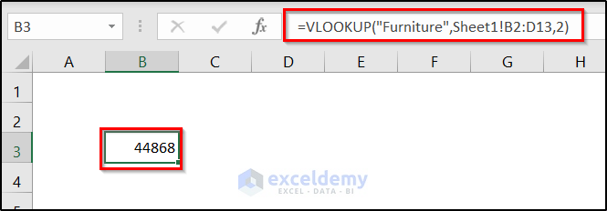
It doesn’t show an accurate result. It is returning the date value in Excel’s format, as we have entered 2 as the return index. And the second column of the table contains date values.
If we enter 3 (as the third column contains the price list) as the col_index_num, it will now provide us with a more accurate result.

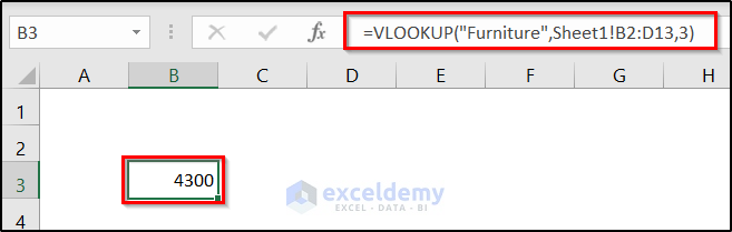
Check for a proper return index. Otherwise, the VLOOKUP will not return the correct value even though it will be picking up the table array either in the same or another worksheet.

Things to Remember

Lock the table array while fetching it within the same workbook.
Remove formulas containing VLOOKUP functions that fetch data from another workbook. As the file paths or directory change, the formula will not function properly in those cases.
Remember to close different instances of Excel workbooks if they are open before working with the formula.
Check for proper arguments and their positions while inserting them into the formula.

Download Practice Workbook

VLOOKUP Not Picking Up Table Array.xlsx

<< Go Back to Issues with VLOOKUP | Excel VLOOKUP Function | Excel Functions | Learn Excel

Get FREE Advanced Excel Exercises with Solutions!