VLOOKUP Not Working (8 Reasons & Solutions)

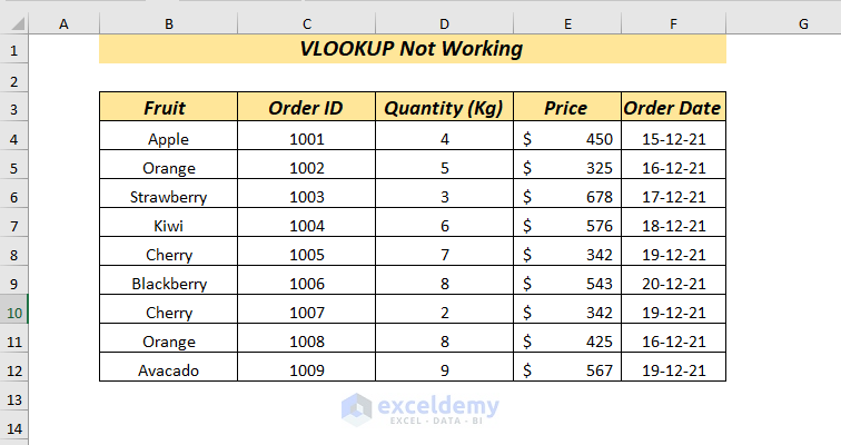
Although VLOOKUP has some limitations, the reason why VLOOKUP is not working is usually human error. To demonstrate the possible issues and their solutions, we’ll use the dataset below.

Download to Practice

8 Reasons Why VLOOKUP is not Working

Case 1 – VLOOKUP Not Working and Showing N/A Error

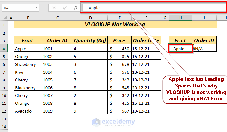
1.1 – Leading and Trailing Spaces 

The possibility of having unwanted spaces in your data is high in a large dataset, and difficult to identify.

Let’s apply the VLOOKUP formula correctly.

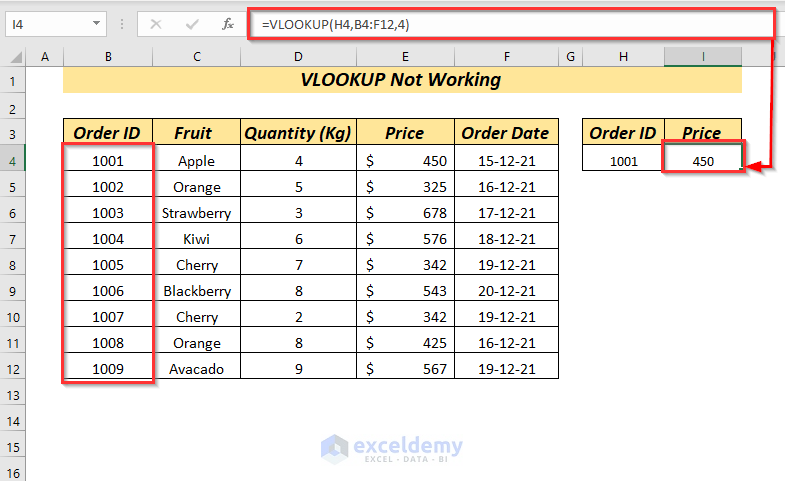
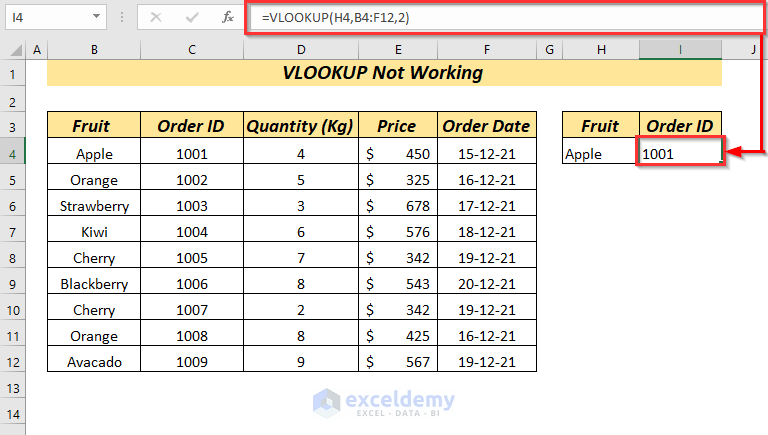
• In cell I4, enter the following formula into the Formula Bar:

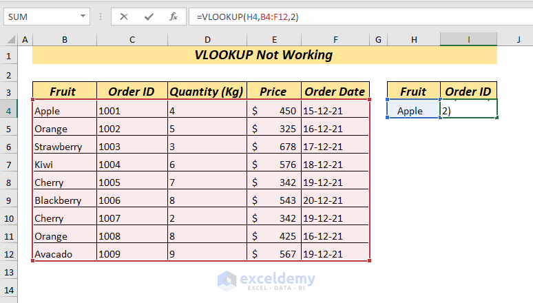
Here, in the VLOOKUP function, we selected the cell H4 as lookup_value, and the range B4:F12 as table_array. As we seek the Order ID, we set 2 as col_index_num.

• Press ENTER.

We were supposed to get the Order ID of the look_up value, but instead we got #N/A.

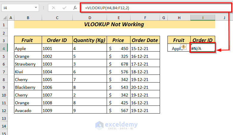
That’s because the lookup_value Apple has some leading spaces.

Solution:

To remove extra leading or trailing spaces, use the lookup_value argument with the TRIM function within the VLOOKUP function.

• Enter the following formula in your selected cell:

The TRIM function will remove all existing leading and trailing spaces of the selected cell H4.

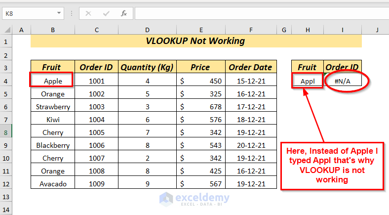
1.2 – Typos

Typing mistakes in the lookup_value will cause VLOOKUP to fail.

Here, we inserted the formula correctly in the selected cell.

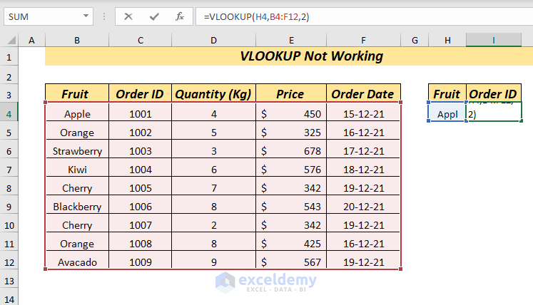
But instead of showing Order ID, it again returns a #N/A error.

The reason is that the spelling of Apple is incorrect, so VLOOKUP can’t make a match.

Solution:

Always carefully type the lookup_value. The string that you are looking for must be identical to the lookup value.

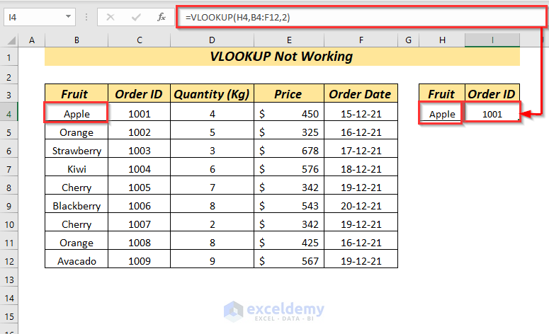
With correct spelling, the formula works as expected.

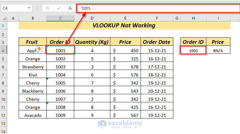
1.3 – Numeric Values Formatted as Text

Numeric values formatted as text in a table_array will return a #N/A error in the VLOOKUP function.

Let’s try to get the Price by using the Order ID as lookup_value.

• In cell I4 enter the following formula into the Formula Bar:

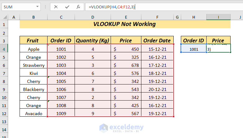
• Press the ENTER key.

We get the #N/A error instead of the expected Price.

That’s because the number 1001 is formatted as text, indicated by the apostrophe before the number.

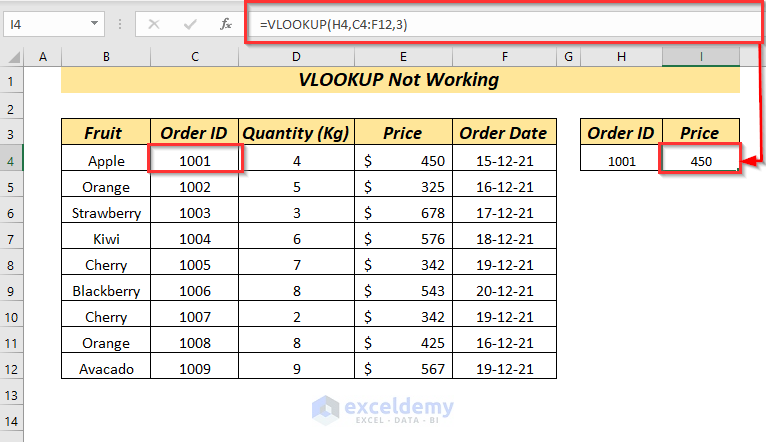
Solution:

Always check the format of the numeric values.

Here, I corrected the numeric format to Number, now the VLOOKUP is working.

Read More: VLOOKUP with Numbers in Excel (4 Examples)

1.4 – Lookup Value is Not in the Leftmost Column

The VLOOKUP function requires the lookup_value to be the leftmost column, or it’ll fail with a #N/A error.

Let’s try to get the Price by using the Order ID as lookup_value.

We use the following formula:

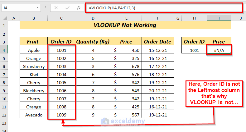
But the Order ID column is not the leftmost column of the table_array B4:F12 so we get a #N/A error back.

Solution:

We can prevent this error in 2 ways:

⏩ Change the table_array so that the lookup_value will be the leftmost column.

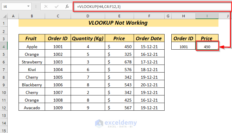
⏩ Place the lookup_value column at the leftmost position of the dataset table.

1.5 – Oversized Table or Inserting New Row & Column with Value

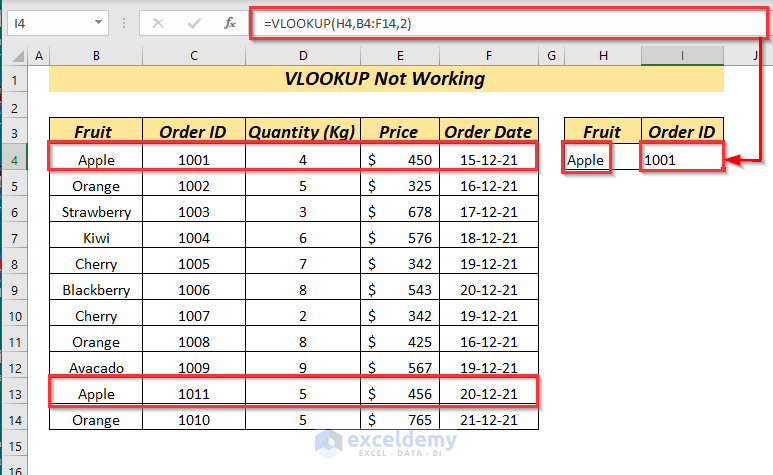
Sometimes we insert new data into our dataset but forget to change the table_array in the VLOOKUP function.

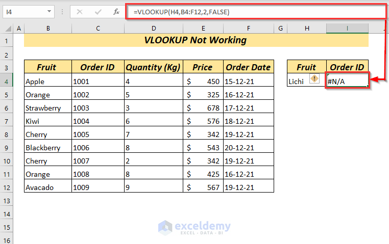
Let’s try to get the Order ID by using the Fruit as lookup_value.

We use the following formula:

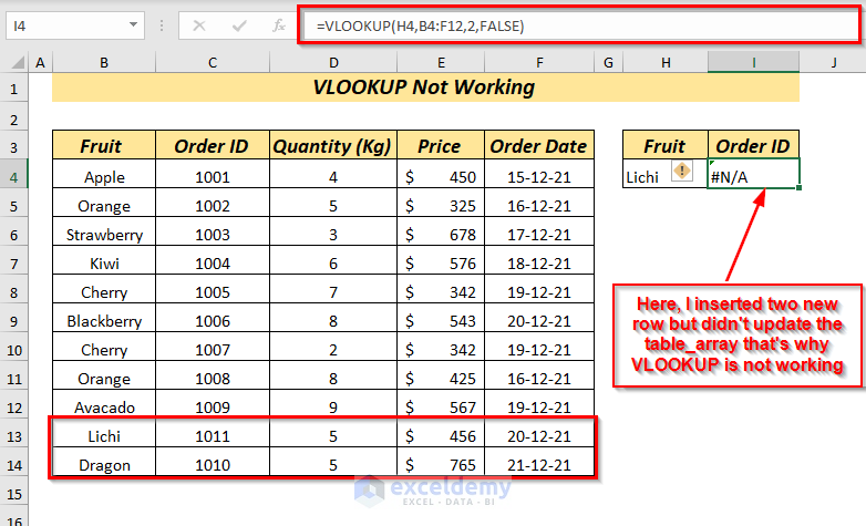
Here, we used the exact match type and looked up Lichi, but received an error, because we didn’t update the table_array to account for two new rows including Lichi that had been added since we inserted the function.

Solution:

Update the table-array whenever you insert new data into your dataset table.

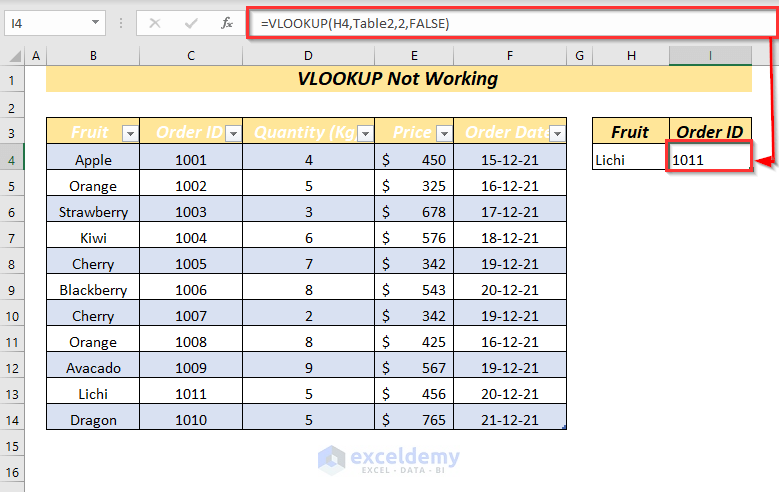
In our example, the function works after we update the table_array in the formula as follows:

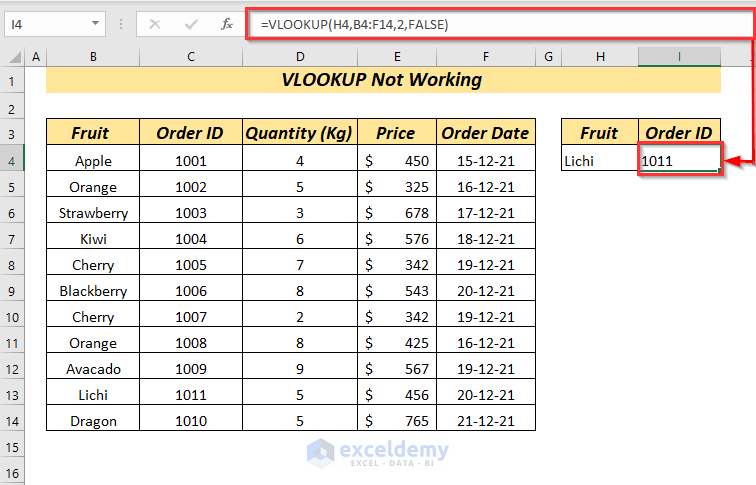
Another solution is converting your dataset into a table.

STEPS:

• Select the cell range.
  Open Insert >> select Table

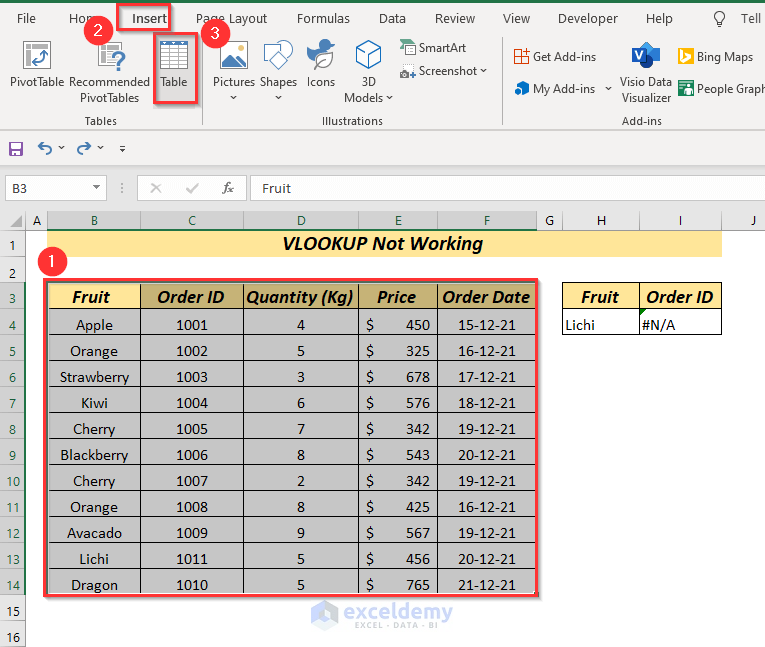
• A dialog box will pop up. Click OK.

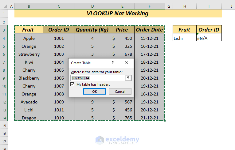
As your dataset is now converted into a table, you can just use the table name in the VLOOKUP function to automatically include any new data.

Read More: How to Use VLOOKUP Function with Exact Match in Excel

Case 2 – VLOOKUP Not Working and Showing VALUE Error

2.1 – For Column Index Number Less than 1

If you mistakenly use a col_index_num less than 1, then you will get #VALUE error.

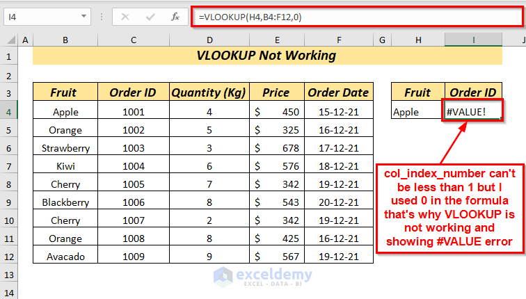
Check your col_index_num argument and adjust as required to solve the problem.

Read More: How to Use Column Index Number Effectively in Excel VLOOKUP

2.2 – Using More than 255 Characters

Lookup text longer than 255 characters will cause a #VALUE error.

Here, in the A7 cell, I inserted a value exceeding 255 characters.

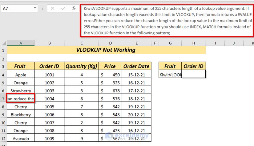
Then, used the following formula:

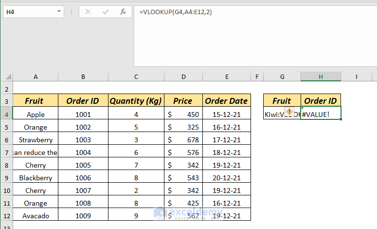
The result is a #VALUE error.

Solution:

Reduce the text length, or use the INDEX and MATCH functions instead of VLOOKUP.

Here, I use the MATCH and the INDEX functions as follows:

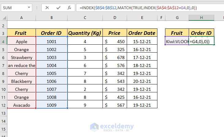
In the INDEX function I selected the absolute reference of the cell range $B$4:$B$12 from where I want to return a value.

In the MATCH function, I set TRUE as the lookup_value and used another INDEX($A$4:$A$12=G4,0) function as lookup_array, then set 0 as match_type to use Exact Match.

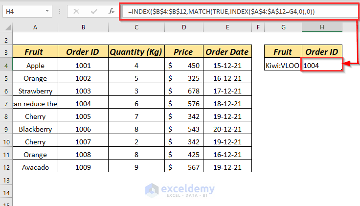
The result is now correct including where the lookup_value is more than 255 characters.

Read More: INDEX MATCH vs VLOOKUP Function (9 Practical Examples)

Case 3 – VLOOKUP Not Working and Showing REF Error

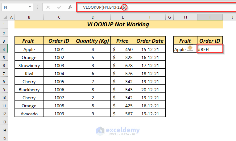
3.1 – Using Column Index Number Greater Than Table

If you use a col_index_num greater than the number of columns in the table_array then you will get #REF error.

Here, I’ve used 6 as col_index_number but the table_array only has 5 columns, which is why the VLOOKUP function is showing a #REF error.

Solution:

Check the col_index_num and use the number which is in the table_array.

Read More: Perform VLOOKUP by Using Column Index Number from Another Sheet

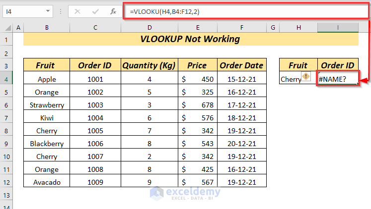
Case 4 – VLOOKUP NAME Error

4.1 – Misspelling the Function Name

The #NAME error is as result of the misspelling of function’s name.

Solution:

Always use the appropriate function name.

Similar Readings

• VLOOKUP from Multiple Columns with Only One Return in Excel
• How to Vlookup with Multiple Matches in Excel (with Easy Steps)
• VLOOKUP and Return All Matches in Excel (7 Ways)
• How to Use VLOOKUP in VBA in Excel (4 Ways)
• VLOOKUP with Drop Down List in Excel

Case 5 – Using Approximate Match

If you use approximate match (TRUE) then there is a possibility of either a #N/A error or incorrect result.

Let’s try to get the Order ID by using the Fruit as lookup_value.

We use the following formula:

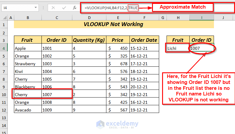
We gave Lichi as lookup_value and used TRUE as range_lookup., but the result shows 1007 as Order ID, which is incorrect because 1007 is the Order ID of Cherry.

Use of approximate match here is the cause of the function returning the wrong information.

Solution:

Use the lookup_value carefully. Instead of using approximate match, use exact match. You may get an error, but that’s much easier to identify and deal with than incorrect information.

You can wrap up the formula with the IFERROR function to show an error message when it can’t find the value within the range.

Read More: 10 Best Practices with VLOOKUP in Excel

Case 6 – Table Reference Is Relative

If your table array is referenced relatively then you may encounter an error notification or error while copying a VLOOKUP formula to lookup other values.

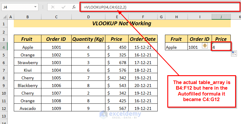
Solution:

Use absolute reference.
Press the F4 key while selecting the reference and it will convert the relative reference to absolute reference.

Here, I used the following formula:

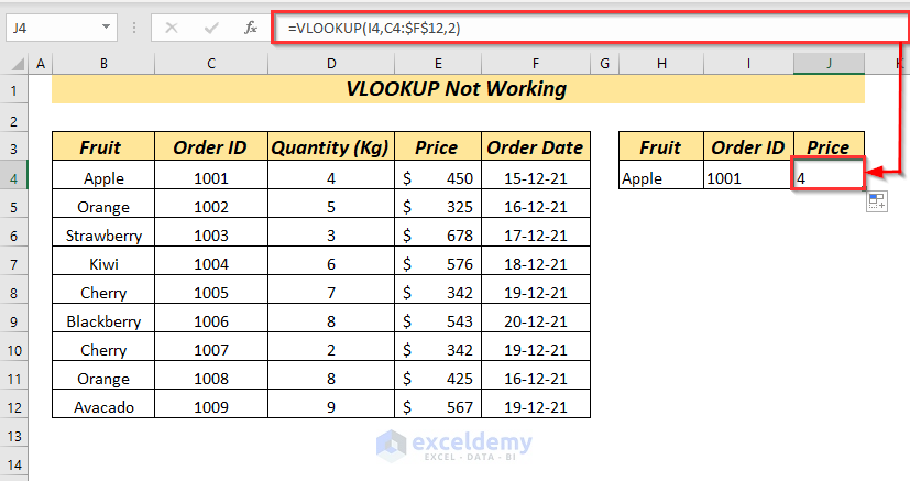
Read More: How to Copy VLOOKUP Formula in Excel (7 Easy Methods)

Case 7 – Inserting a New Column 

If you insert a new column to your existing dataset after applying a VLOOKUP function, it will stop working.

Here, you can see the VLOOKUP function is working properly.

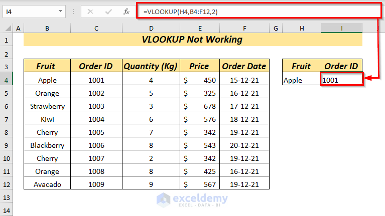
But after I inserted one new column, it is showing 0 instead of the expected result.

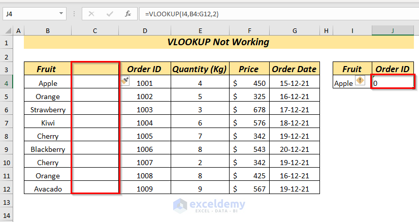
Solution:

⏩ Protect the worksheet.

⏩ Use the MATCH function within the VLOOKUP function.

• Enter the following formula and press Enter.
  
  =VLOOKUP(I4,B4:G12,MATCH(J3,B3:G3,0),FALSE)
  

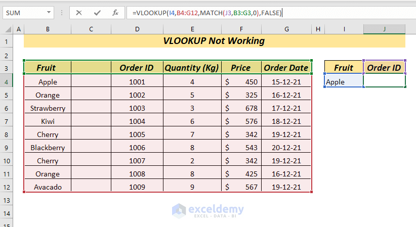
Here, in the VLOOKUP function, we set cell I4 as lookup_value, the range B4:G12 as table_array, the MATCH function as the col_index_num, and FALSE as range_lookup to get Exact Match.

In the MATCH function, we set the column name J3 as lookup_value, the column name range B3:G3 as lookup_array, and 0 as match_type to use Exact Match.

Read More: How to Find Column Index Number in Excel VLOOKUP (2 Ways)

Case 8 – Lookup Value Has Duplicate Values

If your lookup_value contains duplicate values then VLOOKUP won’t work for all the available values. It only returns the value of the first match.

Solution:

Remove the duplicates or you can use the pivot table.

⏩ You can remove the duplicates using Remove Duplicates from then Ribbon.

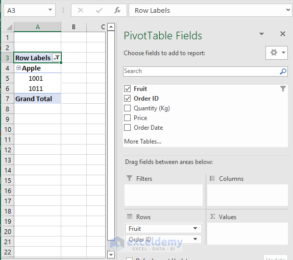
⏩ To use the Pivot Table:

• Select the cell range.
• Open the Insert tab >> select Pivot Table.

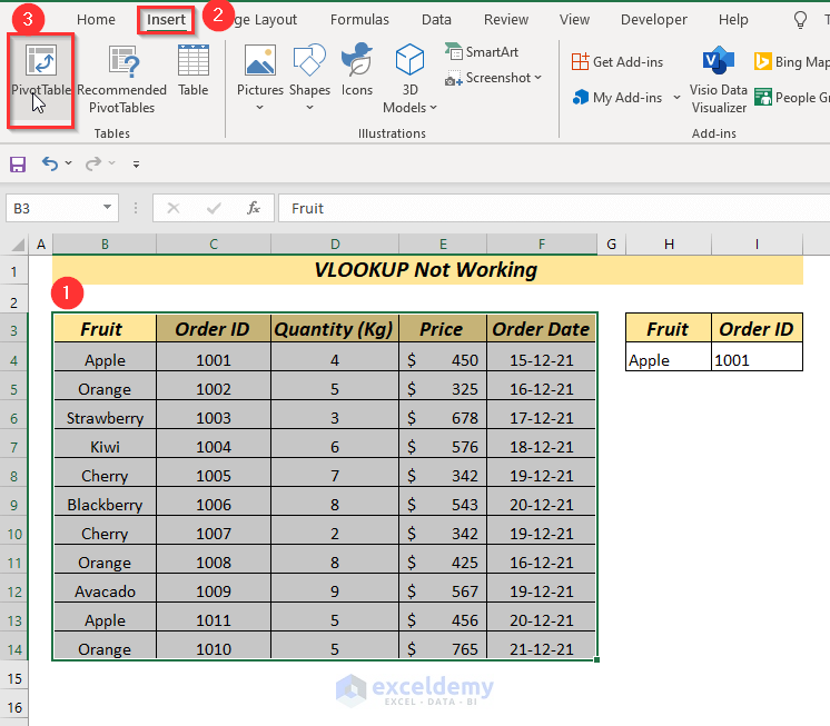
• A dialog box will pop up. Select the place and click OK.

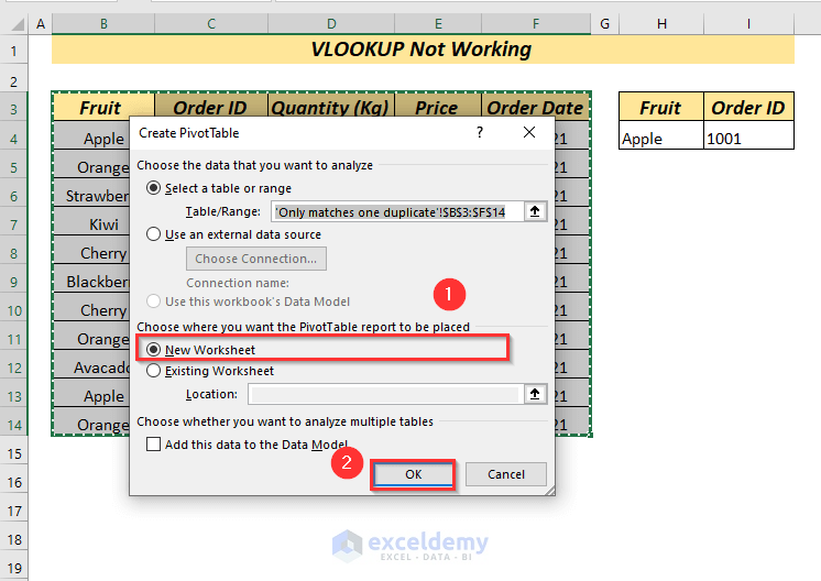
• Select the Fruit and Order ID in Rows and it will show the existing Order ID of your selected Fruit.

Read More: Excel LOOKUP vs VLOOKUP: With 3 Examples

Related Articles

• How to Apply Double VLOOKUP in Excel (4 Quick Ways)
• VLOOKUP with Two Lookup Values in Excel (3 Simple Methods)
• How to Make VLOOKUP Case Sensitive in Excel (4 Methods)
• Use VLOOKUP for Multiple Columns in Excel (6 Examples)
• How to Use Dynamic VLOOKUP in Excel (3 Easy Ways)
• Use VLOOKUP Function in Excel VBA (4 Examples)
• How to Hide VLOOKUP Source Data in Excel (5 Easy Ways)

<< Go Back to Issues with VLOOKUP | Excel VLOOKUP Function | Excel Functions | Learn Excel