How to Vlookup with Multiple Matches in Excel (with Easy Steps)

One of the most amazing and widely used functions of Excel is the VLOOKUP function. So far, we have learned to pull out a single match from a range of cells using this function. You could frequently encounter scenarios in which you need to get all matching values for a unique identifier. In this article, we’ll demonstrate how you can pull out multiple matches from a range of cells using the VLOOKUP function in Excel.

Download Practice Workbook

You may download the following Excel workbook for better understanding and practice yourself.

Performing Vlookup with Multiple Matches.xlsx

2 Steps to Vlookup with Multiple Matches in Excel

Here we have the Book Records of Martin Bookstore. This dataset contains the Book Type, Book Name, and Author of some books under columns B, C, and D correspondingly.

Today our objective is to pull out all the matches of each type of book using the VLOOKUP function. We’ll execute this in two steps. So, let’s explore them one by one.
Here, we have used Microsoft Excel 365 version, you may use any other version according to your convenience.

📌 Step 01: Create Unique Name for Each Lookup Value

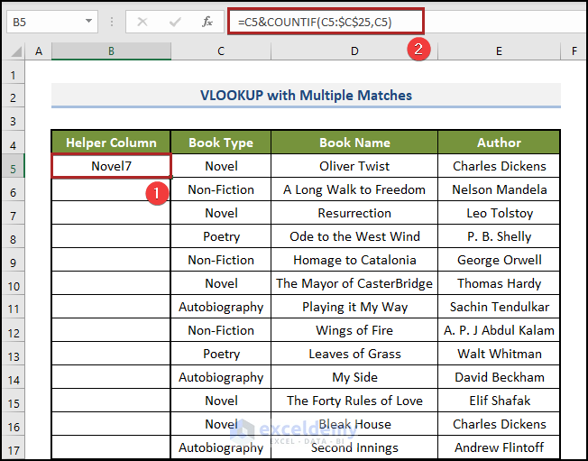
At the very beginning, insert a new column with the heading Helper Column left to the lookup column Book Type and enter this formula in cell B5.

=C5&COUNTIF(C5:$C$25,C5)

Formula Breakdown

COUNTIF(C5:$C$25,C5) returns the total number of cells in the range C5:C25 (Book Type) that contain the value in cell C5 (Novel). See the COUNTIF function for details.
- In simple words, how many novels there are. It is 7.

C5&COUNTIF(C5:$C$25,C5) concatenates the value in cell C5 (Novel) with it.
- So it returns Novel7.

When dragging the Fill Handle tool, C5 increments one by one, like C5, C6, C7… but C25 remains constant. Therefore, for each Book Type, the earlier ones get excluded and a new name is generated.

For example, in the case of novels, Novel1 to Novel7 are generated, and similar for Poetry and other book types.

Then, press ENTER.

After that, bring the cursor to the right-bottom corner of cell B5 and it’ll look like a plus (+) sign. Actually, it’s the Fill Handle tool.
Now, double-click on it.

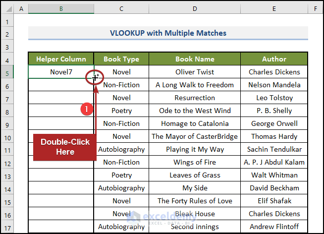
It copies this formula to the rest of the cells. You will find all the lookup values provided with a unique name, like Novel1, Novel2…, Poetry1, Poetry2…, etc.

📌 Step 02: Use VLOOKUP Function

First of all, create a new column with Column Header as the lookup value.

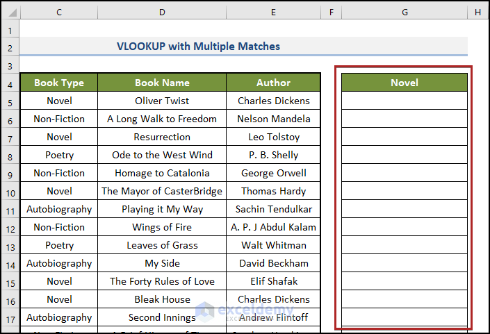
Secondly, insert the following formula in cell G5 which is the first cell of this column.

=VLOOKUP(G$4&ROW($A$1:INDIRECT("A"&COUNTIF($C$5:$C$25,G$4))),$B$5:$E$25,3,FALSE)

Formula Breakdown

COUNTIF($C$5:$C$25,G$4) tells how many cells in the range C5:C25 (Book Type) contain the value in cell G4 (Novel).
- In simple words, how many novels there are in total. It is 7.

We have used the absolute cell reference of the range C5:C25 ($C$5:$C$25) because we want it to remain unchanged if we copy the formula to any cell.

INDIRECT(“A”&COUNTIF($C$5:$C$25,G$4)) becomes INDIRECT(“A”&7) and returns the cell reference A7. See the INDIRECT function for details.
ROW($A$1:INDIRECT(“A”&COUNTIF($C$5:$C$25,G$4))) now becomes ROW(A1:A7).See the ROW function for details.
- It returns an array from 1 to 7 like {1, 2, 3, 4, 5, 6, 7}.

We used $A$1 because we do not want it to change if we copy the formula to another cell.

G$4&ROW($A$1:INDIRECT(“A”&COUNTIF($C$5:$C$25,G$4))) now concatenates the value in cell G4 (Novel) with the array returned by the ROW function and returns another array.
- So it returns {Novel1, Novel2, …, Novel7}.

VLOOKUP(G$4&ROW($A$1:INDIRECT(“A”&COUNTIF($C$5:$C$25,G$4))),$B$5:$E$25,3,FALSE) becomes VLOOKUP({Novel1, Novel2, …, Novel7},$B$5:$E$25,3,FALSE).

It searches for each value of the array {Novel1, Novel2, … Novel7} in the lookup column B.

Then it returns the corresponding name of the novel from the 3rd column (as the col_index_num is 3). Thus, we get a list of all the novels.

As usual, press the ENTER key.

Note: It’s an array formula. So don’t forget to press Ctrl + Shift + Enter unless you are in Excel 365.

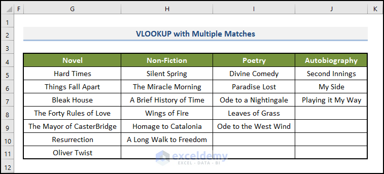
And for the other Book Types,

At first, insert their names side by side as Column Headers and drag the Fill Handle.

Similar Readings

Alternative Ways to Vlookup with Multiple Matches in Excel

If the previous method seems hazardous, don’t worry. There are more options available.

1. Using FILTER Function

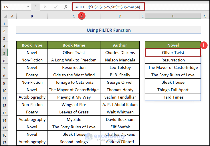
This is indeed the most simple method. Here, we’ll use just the FILTER function. Follow these simple steps.

📌 Steps:

Firstly, write down the Book Type as the Column Header and enter the following formula in cell F5.

=FILTER($C$5:$C$25,$B$5:$B$25=F$4)

Formula Breakdown

Here,

$C$5:$C$25 (Book Name) is the lookup_array. We are looking for the names of the books. You use your one.
$B$5:$B$25 (Book Type) is the matching_array. We want to match the book types. You use your one accordingly.
F4 (Novel) is the matching_value. We want to match the novels. You use it accordingly.

Then, press ENTER.

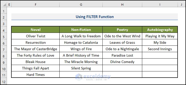
Now, if you want the Book Names of all the Book Types,

Initially, insert their names as the Column Headers side by side, and then drag the Fill Handle tool.

2. Applying Combination of INDEX, SMALL, and ROWS Functions (Compatible with Older Versions of Excel)

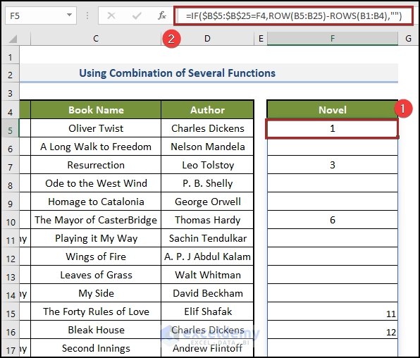
The FILTER function is only available in Office 365. So, if you use the older version of Excel, don’t worry. We have another workaround for you. It’s simple and easy; just follow along.

📌 Steps:

Primarily, insert the Book Type as the Column Header in cell F4 and enter this formula in cell F5.

=IFERROR(INDEX($C$5:$C$25,(SMALL(IF($B$5:$B$25=F4,ROW(B5:B25)-ROWS(B1:B4),""),(ROW(B5:B25)-ROWS(B1:B4))))),"")

Formula Breakdown

ROW(B5:B25) returns an array of {5, 6, 7, …, 25}. And ROWS(B1:B4) returns 4. So ROW(B5:B25)-ROWS(B1:B4) returns an array of {1, 2, 3, …, 21}. See the ROW and ROWS function for details.
IF($B$5:$B$25=F4,ROW(B5:B25)-ROWS(B1:B4),””) returns the corresponding number from the array {1, 2, 3, …, 21} the value in cell F4 (Novel) matches the value in any cell of the range B5:B25 (Book Type). Otherwise returns a blank cell. See the IF function for details.

SMALL(IF($B$5:$B$25=F4,ROW(B5:B25)-ROWS(B1:B4),””),(ROW(B5:B25)-ROWS(B1:B4))) becomes SMALL({1, …, 3, …, 6, …, 20, …},{1, 2, 3, 4, …., 21}) and returns the numbers first, then #NUM! errors in the blank cells. See the SMALL function for details.

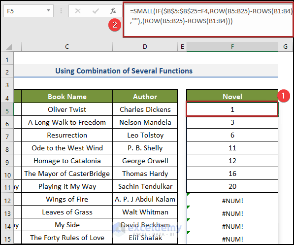
INDEX($C$5:$C$25,(SMALL(IF($B$5:$B$25=F4,ROW(B5:B25)-ROWS(B1:B4),””),(ROW(B5:B25)-ROWS(B1:B4))))) becomes INDEX($C$5:$C$25,{1,3,6,11,…,#NUM!}) and returns the corresponding Book Names (Name of the Novels) and #NUM! errors. See the INDEX function for details.

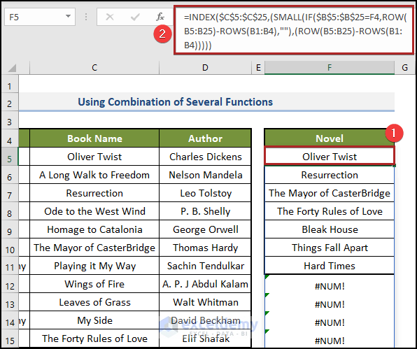
Finally, we wrapped the formula inside an IFERROR function to turn the errors into blank cells.

After that, press ENTER.

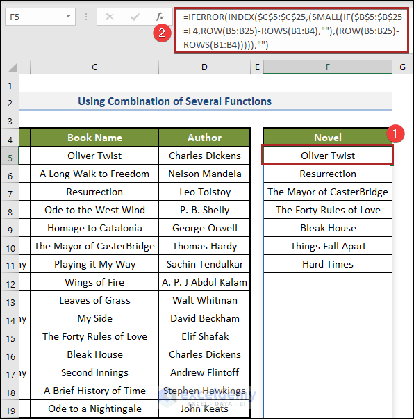
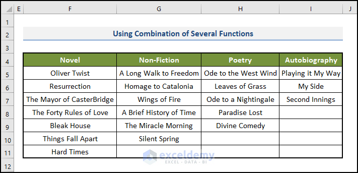
Now, if you want, insert the other Book Types as Column Headers and drag the Fill Handle. You will get the books of the other book types.

3. Vlookup with Multiple Matches and Return Results in a Row

In the previous methods, we got the results in vertical columns. But if we want to get the values in a row, how can we do it? Here, we’ll get the Author names for different Book Types in a row. Just follow the steps below carefully.

📌 Steps:

At first, go to cell G5 and write down the formula below.

=IFERROR(INDEX($D$5:$D$19,SMALL(IF($F5=$B$5:$B$19,ROW($D$5:$D$19)-4,""),COLUMN()-6)),"")

This formula is kind of similar to the previous formula. So, if you face any problem understanding this formula, please see the previous explanation.

Then, tap the ENTER key.

But there are other authors who have novels in this dataset. So, how can we get them?
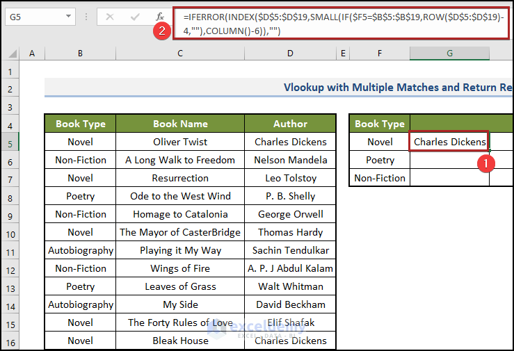
Just drag the Fill Handle to right up to cell K5 to get the other Authors of Novel. Moreover, drag the Fill Handle tool to cell K7 to get the names of Authors for different types of book. See the image below for clarification.

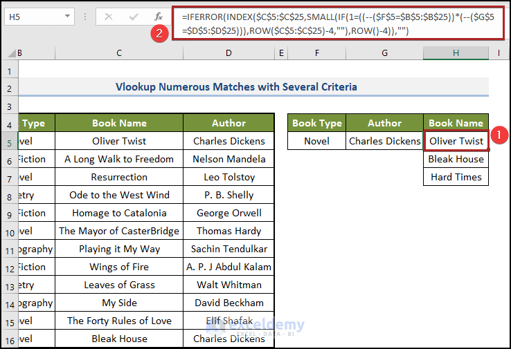
How to Vlookup Numerous Matches with Several Criteria

In our previous examples, we found the values for single criteria. For example, we obtain the titles of books for a specific book type. But here, we’ll imply multiple criteria. We’ll look up the Novels of Charles Dickens using this method. Let’s see it in action.

📌 Steps:

First and foremost, select cell H5 and paste the following formula.

=IFERROR(INDEX($C$5:$C$25,SMALL(IF(1=((--($F$5=$B$5:$B$25))*(--($G$5=$D$5:$D$25))),ROW($C$5:$C$25)-4,""),ROW()-4)),"")

Then, press ENTER.

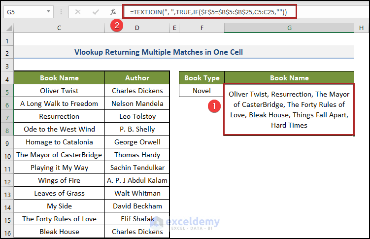
How to Vlookup and Return Multiple Matches in One Cell

In earlier approaches, we got the values in different cells. But we’ll show how we can get results in a single cell. So, without further delay, let’s dive in!

📌 Steps:

Primarily, go to cell G5 and enter the formula below.

=TEXTJOIN(", ",TRUE,IF($F$5=$B$5:$B$25,C5:C25,""))

Here, the IF function gets the value from the range C5:C25 where the corresponding values in the range B5:B25 match the value in cell F5. Then, the TEXTJOIN function combines the values of the array with a comma as the delimiter.

Secondarily, press ENTER.

Conclusion

This article explains how to vlookup with multiple matches in Excel in a simple and concise manner. Don’t forget to download the Practice file. Thank you for reading this article. We hope this was helpful. Please let us know in the comment section if you have any queries or suggestions. Please visit our website, ExcelDemy, a one-stop Excel solution provider, to explore more.

How to Vlookup with Multiple Matches in Excel (with Easy Steps)

Download Practice Workbook

2 Steps to Vlookup with Multiple Matches in Excel

📌 Step 01: Create Unique Name for Each Lookup Value

📌 Step 02: Use VLOOKUP Function

Alternative Ways to Vlookup with Multiple Matches in Excel

1. Using FILTER Function

2. Applying Combination of INDEX, SMALL, and ROWS Functions (Compatible with Older Versions of Excel)

3. Vlookup with Multiple Matches and Return Results in a Row

How to Vlookup Numerous Matches with Several Criteria

How to Vlookup and Return Multiple Matches in One Cell

Conclusion

Further Readings

Leave a reply Cancel reply