Looking for ways to use the VLOOKUP function on multiple rows in Excel? Do not worry, we are here for you. In this article, we will extensively describe how you can use VLOOKUP on multiple rows.
VLOOKUP is an Excel function frequently utilized to locate a particular value within a table and retrieve a matching value from the same row. It can also be used to retrieve values from multiple rows at the same time.
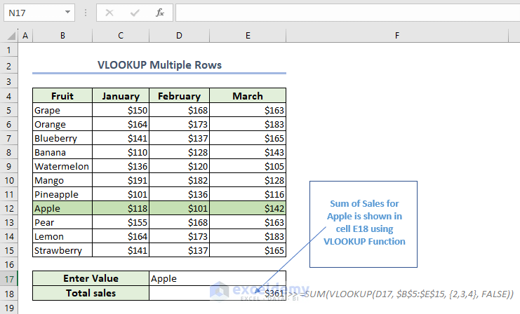
Here, in the following picture, you can see that we have found out the total sales combining 3 rows for the fruit Apple. We have used the VLOOKUP function for this. So let’s dive into the article to find out the ways to do so.
When to Use VLOOKUP for Multiple Rows in Excel?
Below, we are providing some cases when it is necessary to use VLOOKUP for multiple rows.
- Finding Multiple Matching Values: VLOOKUP can help you find many matching values in a big collection of data. For instance, imagine you have a chart with sales information and want to find all the sales made by a particular salesperson. With VLOOKUP, you can extract all the related rows easily.
- Retrieving Specific Information from a Table: VLOOKUP is handy when you want to find certain information from a big table. For instance, suppose you have a list of employees and want to know their salary, department, and job title. You can use VLOOKUP to get this information for each employee.
- Searching Data in Large Dataset: VLOOKUP is a useful tool that saves time when dealing with big sets of data. Instead of searching through the data to find specific information, VLOOKUP lets you easily get the information you need.
How to Use VLOOKUP Function on Multiple Rows in Excel: The Quick Easy Way
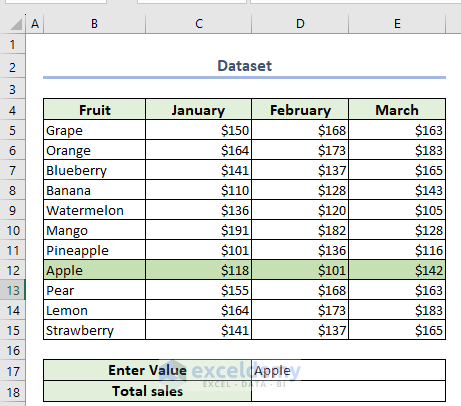
In the following dataset, you can see that we have the Fruit, January, February, and March columns. Using this dataset, we will use VLOOKUP on multiple rows in Excel and find the total according to lookup criteria.
Here, we will mainly find the total sales for the fruit Apple. Thus, we will find the sum of sales for the months of January, February, and March using the VLOOKUP function.
To do so, we have used Microsoft 365. You can use any available Excel version.
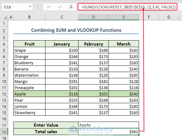
- First of all, we will type the following formula using the SUM and VLOOKUP functions in cells D18:E18.
=SUM(VLOOKUP(D17, $B$5:$E$15, {2,3,4}, FALSE))- After that, we will press ENTER.
As a result, you can see the outcome in cells D18:E18.
Note: Here, each item is presented only once in the Fruit column. This is because the above formula only works when the required item is presented only once in the column.
Formula Breakdown
SUM(VLOOKUP(D17, $B$5:$E$15, {2,3,4}, FALSE))
- The SUM function adds up a range of cells or values.
- The VLOOKUP function looks up a value in the first column of a table or range, and returns a value in the same row from a column you specify.
- D17 is the value being looked up by VLOOKUP.
- $B$5:$E$15 is the range where VLOOKUP looks for the value specified in D17.
- {2,3,4} specifies the columns from which to return values. In this case, the second, third, and fourth columns of the range $B$5:$E$15 will be returned.
- FALSE is an optional parameter that tells VLOOKUP to only return exact matches of the lookup value.
- =SUM(VLOOKUP(D17, $B$5:$E$15, {2,3,4}, FALSE)) → becomes
- Output: $361
An Alternative to Excel VLOOKUP with Multiple Rows Using INDEX-MATCH Formula
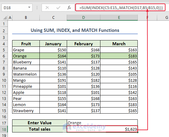
Here, we will use the combination of the SUM, INDEX, and MATCH functions to VLOOKUP multiple rows in Excel.
Here, we will calculate the total sales of Orange using these functions.
- First, we will type the following formula in cells D18:E18.
=SUM(INDEX(C5:E15,,MATCH(D17,B5:B15,0)))- Then, we will press ENTER.
As a result, you can see the outcome in cells D18:E18.
Formula Breakdown
SUM(INDEX(C5:E15,,MATCH(D17,B5:B15,0)))
- The SUM function adds up a range of cells or values.
- The INDEX function returns a value or reference to a cell at the intersection of a specified row and column in a given range.
- C5:E15 is the range from which the values will be selected by INDEX.
- The MATCH function returns the position of a value within an array. In this case, it will find the position of the value in D17 within the range B5:B15.
- D17 is the value being matched by MATCH.
- B5:B15 is the range within which MATCH is searching for a match to D17.
- 0 is an optional parameter that tells MATCH to look for an exact match.
- SUM(INDEX(C5:E15,,MATCH(D17,B5:B15,0))) → becomes
- Output: $1623
Read More: Find Max of Multiple Values by Using VLOOKUP Function in Excel
How to Vlookup and Return Multiple Rows in Excel Using FILTER Function
Here, we will use the FILTER function to return multiple rows in Excel. One thing must be remembered, that the FILTER function is only available in Microsoft 365.
Using the FILTER function for our dataset, we will return the rows with Vegetables in them.
- In the beginning, we will type the following formula in cell D18.
=FILTER(B5:D15,C5:C15=D17)The FILTER function filters a range of values in a dataset based on certain criteria.
- After that, we will press ENTER.
As a result, you can see the outcome in cells D18:F19.
How to Use VLOOKUP Based on Multiple Criteria in Excel
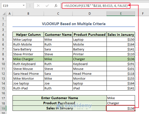
Here, we will use VLOOKUP based on multiple criteria.
For our dataset, we have set the criteria as Mike and Charger in cells E17 and E18. Now, we will find out Sales in January based on these criteria.
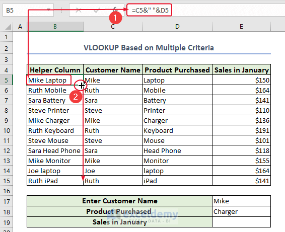
- First of all, we will insert a Helper Column.
- We will type the following formula in cell B5.
=C5&" "&D5- We will drag down the formula with the Fill Handle tool.
Therefore, you can see the complete Helper Column.
- After that, we will type the following formula in cell E19.
=VLOOKUP(E17&" "&E18, B5:E15, 4, FALSE)- Then, press ENTER.
As a result, you can see the result in cell E19.
Read More: How to VLOOKUP Multiple Values in One Cell in Excel
How to VLOOKUP in Both Rows and Columns in Excel (Two-Way Lookup)
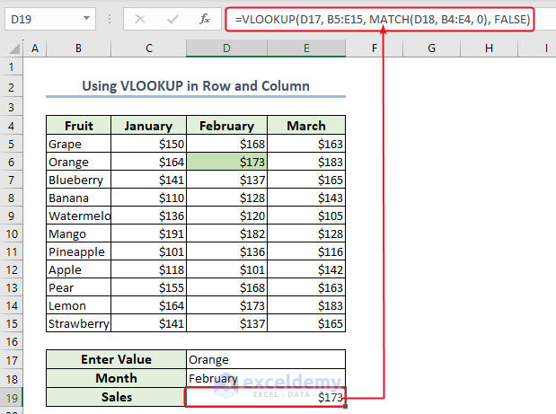
Here, we will use the VLOOKUP and MATCH functions to find out the Sales of Orange for the month of February. Thus, we have to VLOOKUP from rows and columns, which is a two-way lookup.
- In the first place, we will type the following formula in cells D19:E19.
=VLOOKUP(D17, B5:E15, MATCH(D18, B4:E4, 0), FALSE)- After that, press ENTER.
Therefore, you can see the result in cells D19:E19.
How to Use VLOOKUP to Return Nth Match in Excel
If you have a dataset, where you have repetitive matches, and you want to return Nth match, you can do so using the VLOOKUP function.
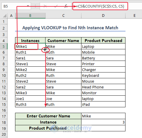
In the following dataset, you can see that we have repetitive Customer Names. Now, we will find out the Product Purchased for customer Mike for the 3rd match.
You can see the Customer Name in cell D17, and the Instance in cell D18.
Now, to find the Product Purchased we need to insert an Instances column.
- First of all, we will type a formula including the COUNTIF function in cell B5.
=C5&COUNTIF($C$5:C5, C5)The COUNTIF function calculates a range of cells based on criteria.
- At this point, press ENTER.
As a result, you can see the outcome in cell B5.
- Now, we will drag down the formula with the Fill Handle tool.
As a result, you can see the complete Instances column.
- After that, we will type the following formula in cell D19.
=VLOOKUP(D17&D18, B5:D15, 3, FALSE)- After that, press ENTER.
Therefore, you can see the result in cell D19.

Things to Remember
- You must be sure of what value you are searching for.
- Insert a Helper column whenever you want to find the Nth match or use VLOOKUP for multiple criteria.
- Check function syntax properly.
Download Practice Workbook
You can download the Excel file from the link below and practice the explained methods.
Conclusion
In this article, we extensively describe how to use the VLOOKUP function on multiple rows in Excel. We describe an easy and quick way for this.
In addition to this, we describe how you can return multiple rows using the FILTER function.
Also, we describe how you can use VLOOKUP based on multiple criteria, in rows and columns (two ways lookup), and to return Nth match.
Thank you for going through the article. We hope it was helpful. If you have any queries or suggestions, please let us know in the comment section.
Related Articles
- Excel VLOOKUP to Return Multiple Values in One Cell Separated by Comma
- VLOOKUP to Return Multiple Values Horizontally in Excel
- How to Use Excel VLOOKUP to Return Multiple Values Vertically
- How to Vlookup and Return Multiple Values in Drop Down List
<< Go Back to VLOOKUP Multiple Values | Excel VLOOKUP Function | Excel Functions | Learn Excel
Get FREE Advanced Excel Exercises with Solutions!
