Method 1 – Combining the VLOOKUP and the MAX Functions to Find the Max of Multiple Values
This is the sample dataset.
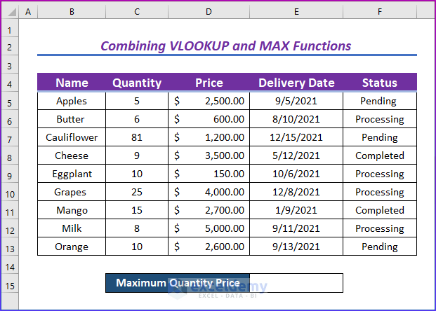
Steps:
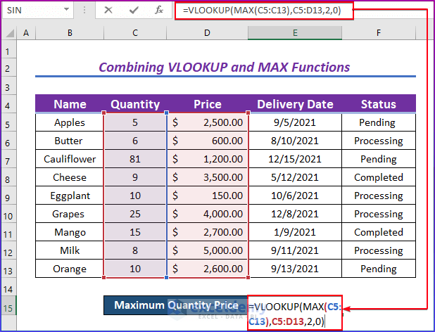
- Enter the following formula in E15.
=VLOOKUP(MAX(C5:C13),C5:D13,2,0)- Press Enter.
Formula Breakdown
- VLOOKUP (value, table, col_index, [range_lookup]) this is the syntax of the VLOOKUP function, in which MAX (C5:C13) is the value, C5:D13 is the table, 2 is the col_index, and 0 is [range_lookup].
- MAX(C5:C13) is the lookup value.
- C5:D13 is the table array.
- The column index number was used as there are 2 columns.
- 0 is used for an exact match.
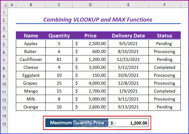
This is the output.
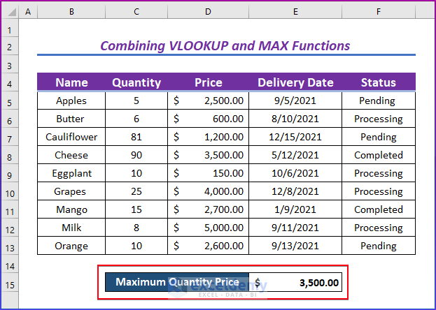
You can change values in the quantity column and see the change in the output box. Here, the Cheese quantity was changed from 9 to 90.
The maximum quantity price automatically changes.
Read More: How to VLOOKUP Multiple Values in One Cell in Excel
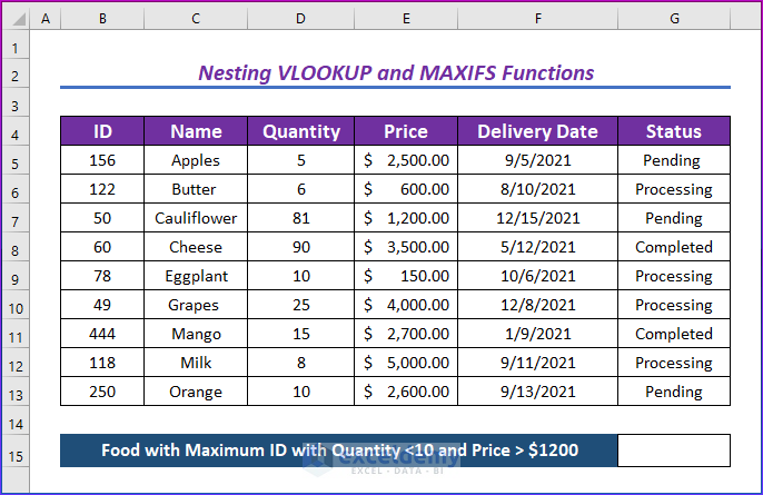
Method 2 – Nesting the VLOOKUP and the MAXIFS Functions to Find the Max Value with Multiple Criteria
Find the name of the food with a maximum ID, a quantity less than 10, and a price greater than $1,200.
Steps:
- Enter the following formula in G14.
=VLOOKUP(MAXIFS(B5:B13,D5:D13,"<10",E5:E13,">1200"),B5:G13,2,FALSE)- Press Enter.
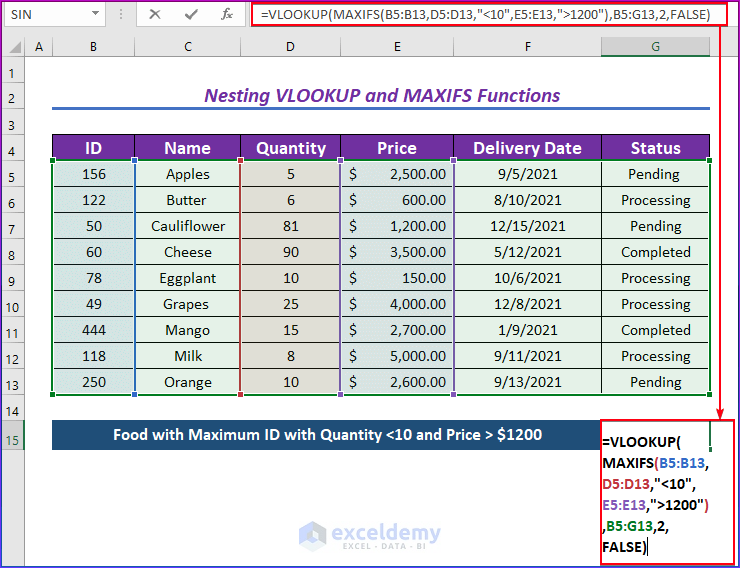
Formula Breakdown
- MAXIFS(B5:B13,D5:D13,”<10″,E5:E13,”>1200″) returns the maximum ID number with a quantity less than 10 and a price greater than $1200.
- The VLOOKUP function returns the Name of the matched ID. Here, 2 is used, as the name is in the second column. FALSE or 0 is used to get an exact match.
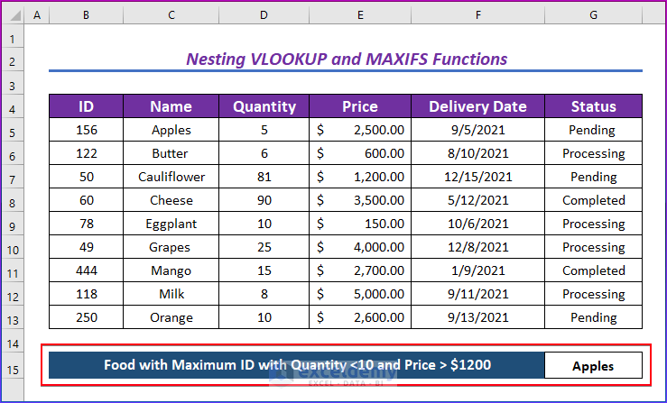
This is the output.
Read More: VLOOKUP to Return Multiple Values Horizontally in Excel
The VLOOKUP Function Is Not Working in Excel – Reasons
| Common Errors | When they show |
|---|---|
| #N/A | If the lookup_value is smaller than the smallest value in the first column of the table_array, you’ll see the #N/A error value.#REF! |
| #REF! | If the col_index_num is greater than the number of columns in table array, you’ll get the #REF! error value. |
| #VALUE! | If the table_array is less than 1, you’ll get the #VALUE! error value. |
| #NAME? | The #NAME? error value means the formula is missing quotes. |
| #SPILL! | The #SPILL! error means the formula is relying on the implicit intersection for the lookup value and using an entire column as a reference. |
- To declare a match type, use 1/0 or TRUE/FALSE.
- If the range_lookup is TRUE or left out, the first column needs to be sorted alphabetically or numerically. Either sort the first column or use FALSE for an exact match.
Download the Practice Workbook
Related Articles
- How to Use Excel VLOOKUP to Return Multiple Values Vertically
- How to Use VLOOKUP Function on Multiple Rows in Excel
- How to Vlookup and Return Multiple Values in Drop Down List
- Excel VLOOKUP to Return Multiple Values in One Cell Separated by Comma
<< Go Back to VLOOKUP Multiple Values | Excel VLOOKUP Function | Excel Functions | Learn Excel
Get FREE Advanced Excel Exercises with Solutions!
