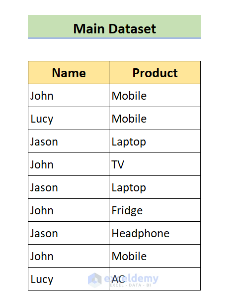
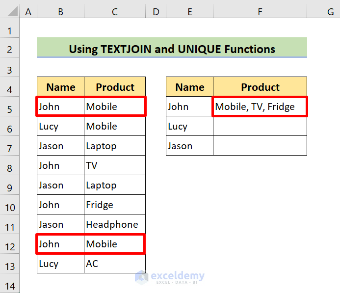
We have a dataset with salesperson Names and their selling Products. Our goal is to find the selling products of each salesperson.
Method 1 – Using Formulas to Vlookup Multiple Values in One Cell in Excel
The TEXTJOIN function will be used for this method. The TEXTJOIN function allows you to join 2 or more strings together with each value separated by a delimiter.
The Basic Syntax of TEXTJOIN Function:
=TEXTJOIN(delimiter, ignore_empty, text1, [text2], …)The delimiter will be a comma (“,”) to separate values in one cell.
1.1 The TEXTJOIN and IF Functions
The Basic Syntax:
=TEXTJOIN(", ",TRUE,IF(lookup_value=lookup_range,,finding_range,""))Steps
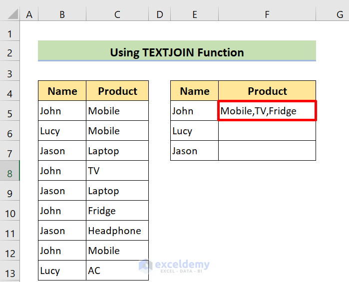
- Enter the following formula in Cell F5:
=TEXTJOIN(", ",TRUE,IF(E5=B5:B13,C5:C13,""))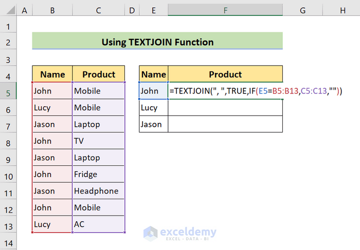
2. Press Enter.
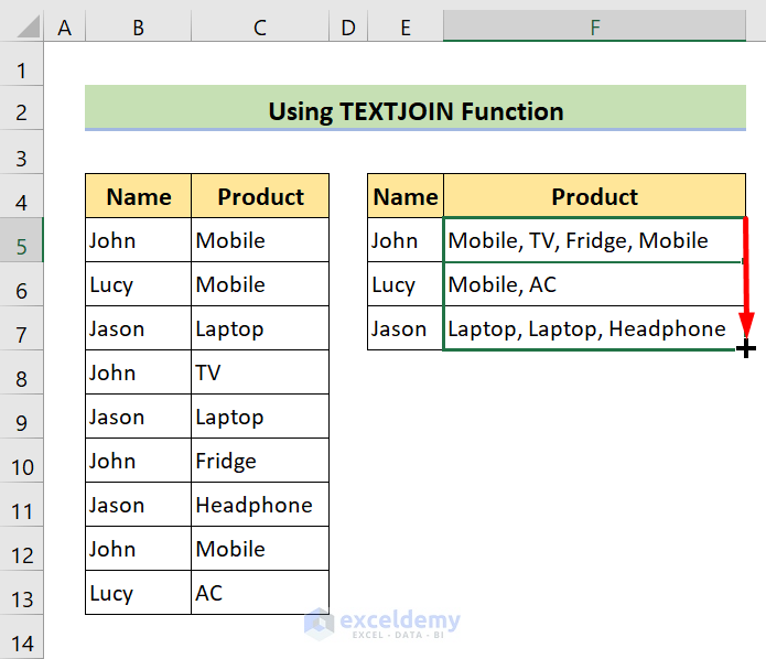
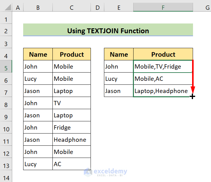
3. Drag the Fill Handle icon to fill in the remaining cells.
Breakdown of the Formula
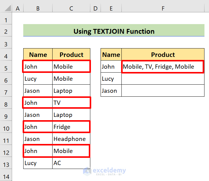
We are using this breakdown only for the person “John”
➤ IF(E5=B5:B13,C5:C13,"")
This function returns the following array:
{"Mobile";"";"";"TV";"";"Fridge";"";"Mobile";""}
➤ TEXTJOIN(", ",TRUE,IF(E5=B5:B13,C5:C13,""))
The TEXTJOIN function will return the following result:
{Mobile, TV, Fridge, Mobile}
Read More: Excel VLOOKUP to Return Multiple Values in One Cell Separated by Comma
1.2 The TEXTJOIN and MATCH Functions (Without Duplicates)
STEPS
1. Enter the following formula in cell F5:
=TEXTJOIN(",", TRUE, IF(IFERROR(MATCH(C5:C13, IF(E5=B5:B13, C5:C13, ""), 0),"")=MATCH(ROW(C5:C13), ROW(C5:C13)), C5:C13, ""))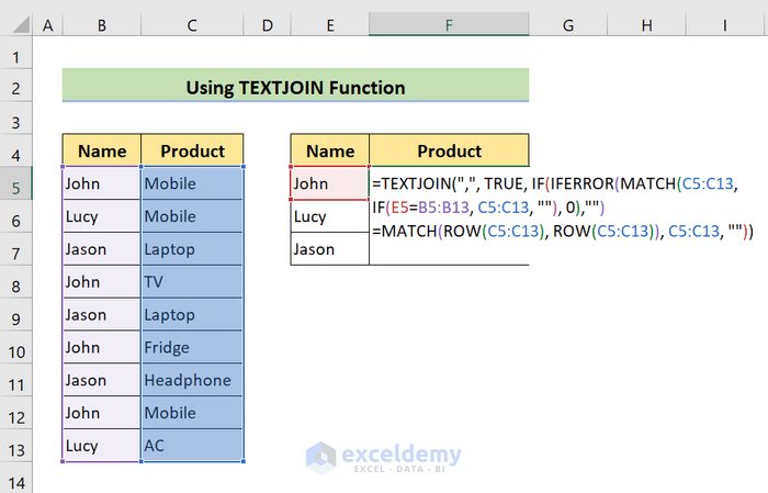
2. Press Enter.
3. Drag the Fill Handle icon to fill in the remaining cells.
Breakdown of the Formula
We are using this breakdown only for the person “John”
➤ ROW(C5:C13)
It returns an array of {5;6;7;8;9;10;11;12;13}
➤ MATCH(ROW(C5:C13), ROW(C5:C13))
It returns: {1;2;3;4;5;6;7;8;9}
➤ IF(E5=B5:B13, C5:C13, "")
It returns: {"Mobile";"";"";"TV";"";"Fridge";"";"Mobile";""}
➤ MATCH(C5:C13, IF(E5=B5:B13, C5:C13, "")
This function returns: {8;8;7;9;7;7;7;8;7}
➤ IFERROR(MATCH(C5:C13, IF(E5=B5:B13, C5:C13, ""), 0),"")
It returns: {1;1;"";4;"";6;"";1;""}
➤ IF(IFERROR(MATCH(C5:C13, IF(E5=B5:B13, C5:C13, ""), 0),"")=MATCH(ROW(C5:C13), ROW(C5:C13)), C5:C13, "")
It returns: {"Mobile";"";"";"TV";"";"Fridge";"";"";""}
➤ TEXTJOIN(",", TRUE, IF(IFERROR(MATCH(C5:C13, IF(E5=B5:B13, C5:C13, ""), 0),"")=MATCH(ROW(C5:C13), ROW(C5:C13)), C5:C13, ""))
The final output will be Mobile, TV, Fridge.
Read More: How to Use VLOOKUP Function on Multiple Rows in Excel
1.3 The TEXTJOIN and UNIQUE Functions (Without Duplicates)
The Basic Syntax of UNIQUE Function:
=UNIQUE (array, [by_col], [exactly_once])array – Range or array from which to extract unique values.
by_col – [optional] How to compare and extract. By row = FALSE (default); by column = TRUE.
exactly_once – [optional] TRUE = values that occur once, FALSE= all unique values (default)
STEPS
1. Enter the following formula in cell F5:
=TEXTJOIN(", ",TRUE,UNIQUE(IF(E5=B5:B13,C5:C13,"")))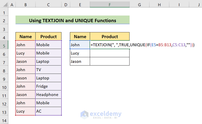
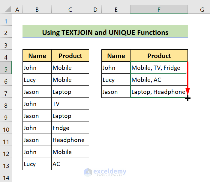
2.Press Enter.
3. Drag the Fill Handle icon to fill in the remaining cells.
Breakdown of the Formula
We are using this breakdown only for the person “John”
➤ IF(E5=B5:B13,C5:C13,"")
It returns {"Mobile";"";"";"TV";"";"Fridge";"";"Mobile";""}
➤ UNIQUE(IF(E5=B5:B13,C5:C13,""))
It returns {"Mobile";"";"TV";"Fridge"}
➤ TEXTJOIN(", ",TRUE,UNIQUE(IF(E5=B5:B13,C5:C13,"")))
Final result Mobile,TV,Fridge
Read More: How to Vlookup and Return Multiple Values in Drop Down List
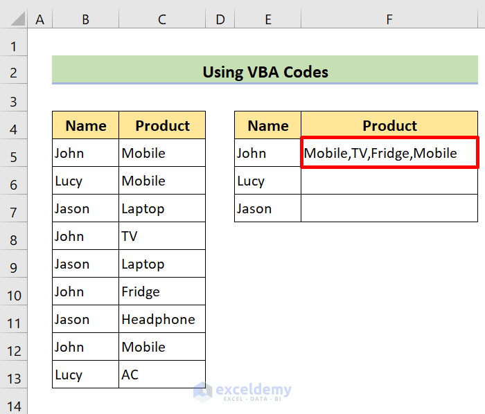
Method 2 – Using VBA Codes to Vlookup Multiple Values in One Cell
2.1 VBA Codes Multiple Values in One Cell
STEPS
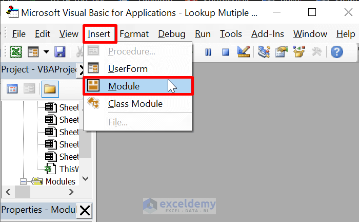
1. Press Alt+F11 to open Visual Basic Editor.
2. Click on Insert > Module.
3. Enter the following code:
Function MultipleValues(work_range As Range, criteria As Variant, merge_range As Range, Optional Separator As String = ",") As Variant
Dim outcome As String
On Error Resume Next
If work_range.Count <> merge_range.Count Then
MultipleValues = CVErr(xlErrRef)
Exit Function
End If
For i = 1 To work_range.Count
If work_range.Cells(i).Value = criteria Then
outcome = outcome & Separator & merge_range.Cells(i).Value
End If
Next i
If outcome <> "" Then
outcome = VBA.Mid(outcome, VBA.Len(Separator) + 1)
End If
MultipleValues = outcome
Exit Function
End Function
4. Go to your worksheet and enter the following formula in Cell F5:
=MultipleValues(B5:B13,E5,C5:C13,",")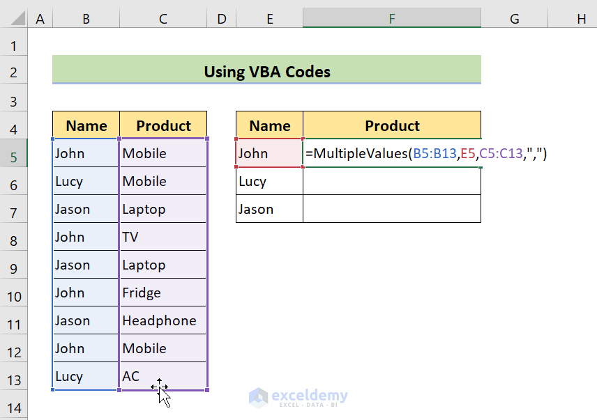
5. Press ENTER.
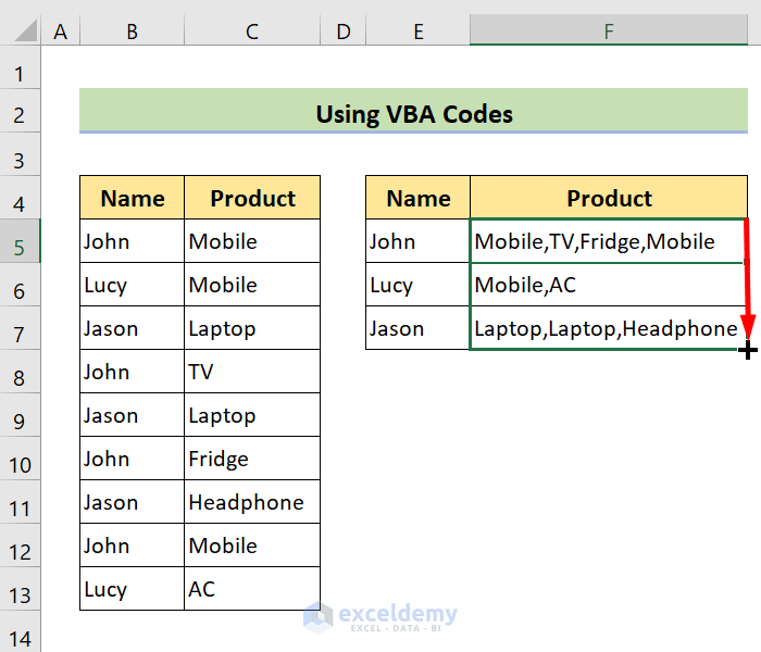
6. Drag the Fill Handle icon to fill in the remaining cells.
Read More: VLOOKUP to Return Multiple Values Horizontally in Excel
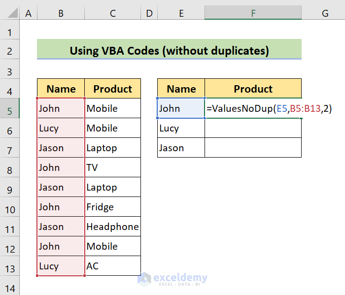
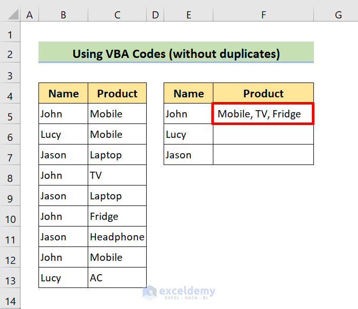
2.2 VBA Codes to LOOKUP Multiple Values in One Cell (Without Duplicates)
STEPS
1. Press Alt+F11 to open Visual Basic Editor.
2. Click on Insert > Module.
3. Enter the following code:
Function ValuesNoDup(target As String, search_range As Range, ColumnNumber As Integer)
Dim i As Long
Dim outcome As String
For i = 1 To search_range.Columns(1).Cells.Count
If search_range.Cells(i, 1) = target Then
For J = 1 To i - 1
If search_range.Cells(J, 1) = target Then
If search_range.Cells(J, ColumnNumber) = search_range.Cells(i, ColumnNumber) Then
GoTo Skip
End If
End If
Next J
outcome = outcome & " " & search_range.Cells(i, ColumnNumber) & ","
Skip:
End If
Next i
ValuesNoDup = Left(outcome, Len(outcome) - 1)
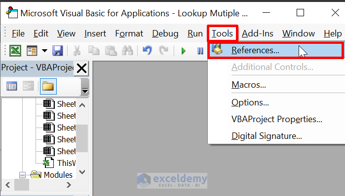
End Function4. The Microsoft Visual Basic for Applications window will open. Click Tools > References. From the References – VBAProject dialog box, check the Microsoft Scripting Runtime option in the Available References list box. Click OK.

5. Go to the worksheet and enter the following formula in Cell F5:
=ValuesNoDup(E5,B5:B13,2)2 is the column number of the dataset.
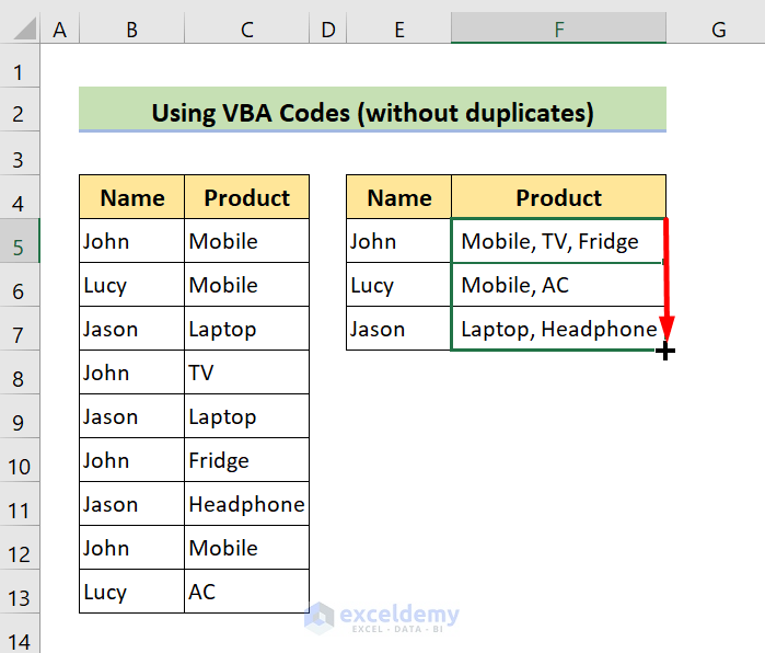
6. Press Enter.
7. Drag the Fill Handle icon to fill in the remaining cells.
Download Practice Workbook
Related Articles
- Find Max of Multiple Values by Using VLOOKUP Function in Excel
- How to Use Excel VLOOKUP to Return Multiple Values Vertically
<< Go Back to VLOOKUP Multiple Values | Excel VLOOKUP Function | Excel Functions | Learn Excel
Get FREE Advanced Excel Exercises with Solutions!

Awesome tutorial. I’m always forgetting how to find and add multiple data points to one cell, especially when I have to create a specialized list using our directory of 8K employees. I have now downloaded the file and saved the formulas for quick reference. Thank you!
Hello NadineB,
You are most welcome. Thanks a lot for your appreciation.
Regards
ExcelDemy