Problems with the VLOOKUP When Returning Multiple Matches:
In the dataset below there are three columns: Book Type, Book Name, and Author.
To get the names of all autobiographies using the VLOOKUP formula, you will get only one book name when there are 2.
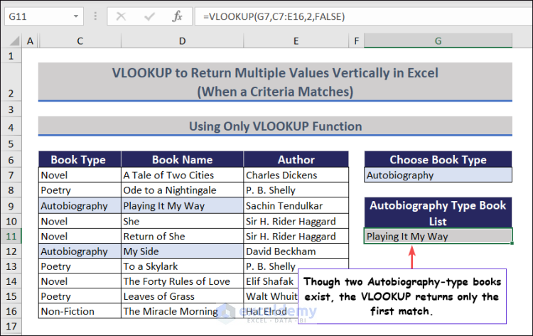
In the following image the formula returned the correct result.

Overview of Excel VLOOKUP to Return Multiple Values Vertically
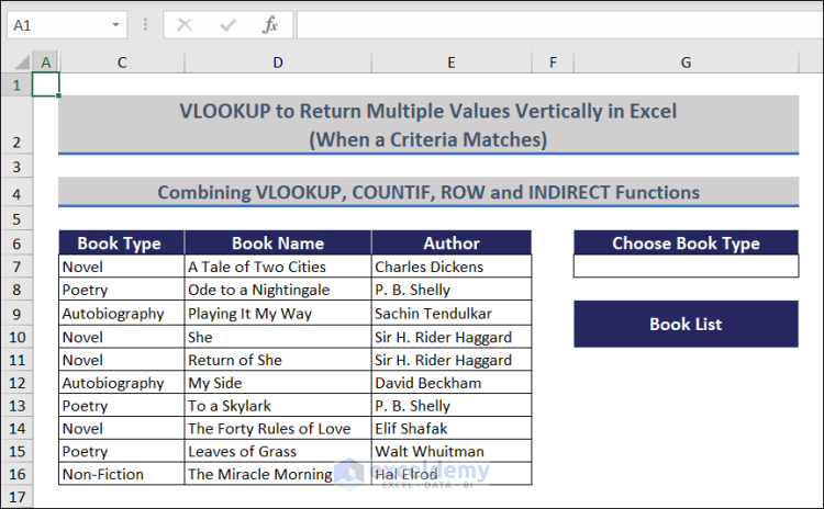
Method 1 – Combining the VLOOKUP, COUNTIF, ROW and INDIRECT Functions to Return Multiple Values Vertically
The dataset has three columns: Book Type, Book Name, and Author.
Step 1:
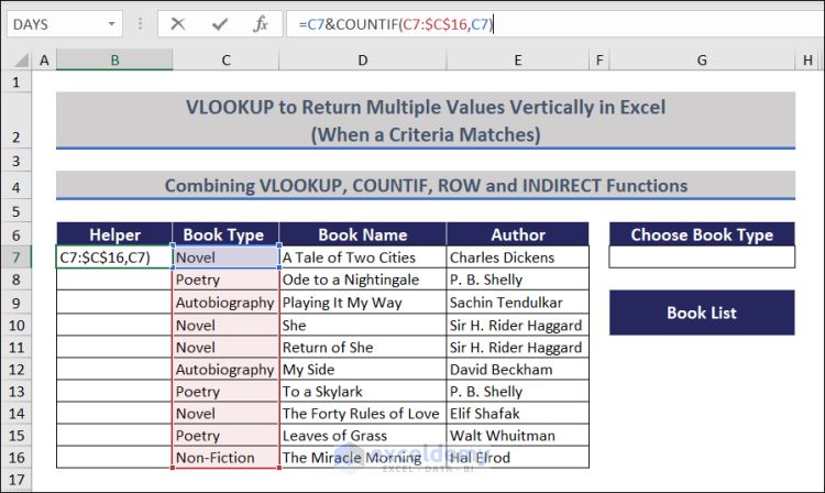
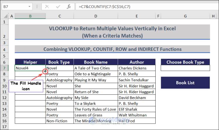
- Insert a helper column. Select B7 and enter the following formula.
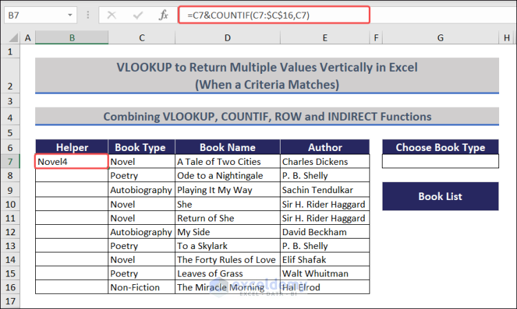
=C7&COUNTIF(C7:$C$16,C7)
Step 2:
- Press Enter.
You will see Novel4 in B7.
Step 3:
- Place the cursor at the bottom right corner of B7. You will see the Fill Handle icon.
Step 4:
- Drag down the Fill Handle to see the result in the rest of the cells. The helper column is created.
![]()
Step 5:
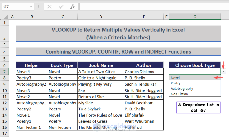
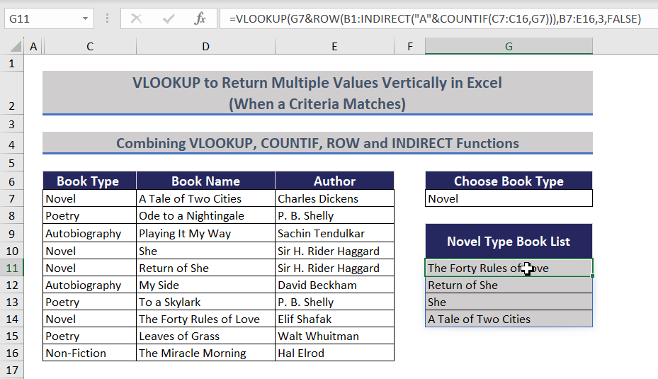
- Select G7. Create a drop-down to choose the book type .
- Click the drop-down and choose Novel.
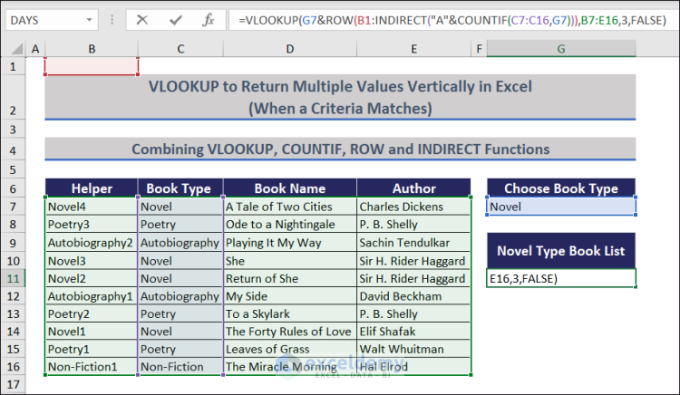
Step 6:
- Choose G11 and enter the following formula.
=VLOOKUP(G7&ROW(B1:INDIRECT("A"&COUNTIF(C7:C16,G7))),B7:E16,3,FALSE)
Step 7:
- Press Enter to see the output.
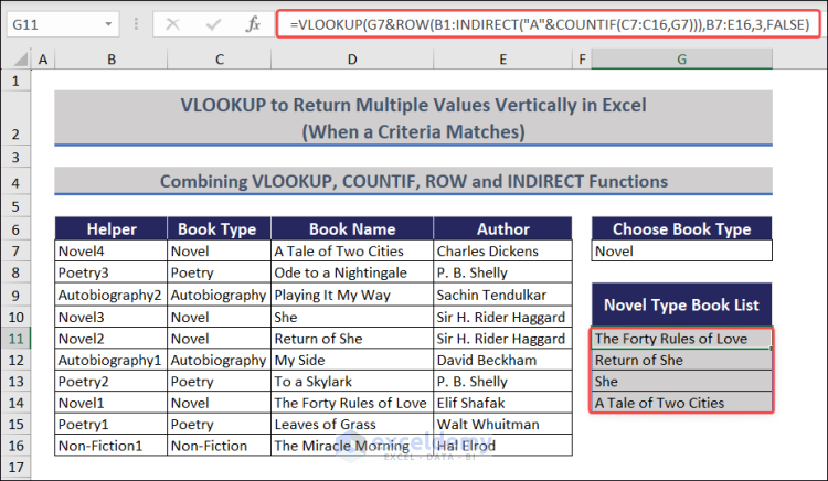
A column header is created for the Book List column. It will change based on the value entered in G7. Conditional Formatting is used to highlight and create borders in the output.
Step 8:
If you change the book type in the drop-down list, the names will be returned and highlighted.
Observe the GIF.
The helper column was hidden.
=VLOOKUP(G7&ROW(B1:INDIRECT(“A”&COUNTIF(C7:C16,G7))),B7:E16,3,FALSE)
=VLOOKUP(G7&ROW(B1:INDIRECT(“A”&2)),B7:E16,3,FALSE) // COUNTIF(C7:C16,G7) counts if the value of G7 is found in C7:C16. For example, if the value of G7 is Autobiography, we will get 2.
=VLOOKUP(G7&ROW(B1:INDIRECT(“A”&2)),B7:E16,3,FALSE)
=VLOOKUP(G7&ROW(B1:0),B7:E16,3,FALSE) // INDIRECT(“A”&1)) returns the values of A1.
=VLOOKUP(G7&ROW(B1:0),B7:E16,3,FALSE)
=VLOOKUP(G7&{1;2},B7:E16,3,FALSE) // ROW(B1:0) returns {1;2}.
=VLOOKUP(G7&{1;2},B7:E16,3,FALSE)
=VLOOKUP({“Autobiography1″;”Autobiography2”},B7:E16,3,FALSE) // G7&1 returns {“Autobiography1″;”Autobiography2”}.
=VLOOKUP({“Autobiography1″;”Autobiography2”},B7:E16,3,FALSE)
={“My Side”;”Playing It My Way”} // VLOOKUP({“Autobiography1″;”Autobiography2”}, B7:E16,3,FALSE) searches “Autobiography1” and “Autobiography2” in column B and returns the corresponding values in column D.
Method 2 – Using the VLOOKUP, FILTER, and IFS Functions to Return Multiple Values Vertically
The dataset showcases Book Type, Book Name, and Sales Quantity.
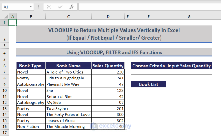
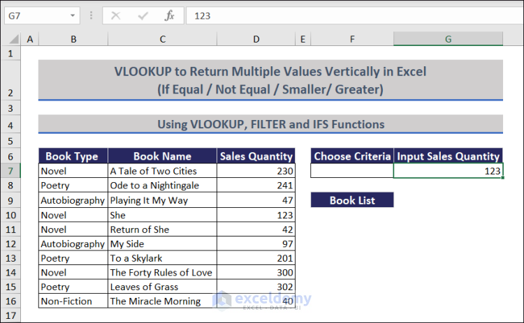
Step 1:
- Select G7 => Enter 123 in Sales Quantity.
Step 2:
- Select F7 => Create a drop-down to choose <, >, =, or <> signs => Expand the drop-down => Choose Greater Than (>) sign.
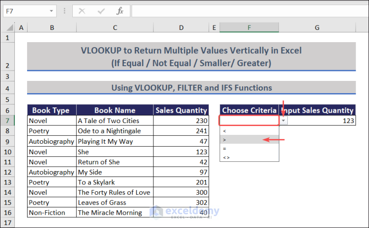
While creating the drop-down, do not enter the Equal (=) sign at the beginning in the Source field.
Step 3:
- Select F10 => Enter the following formula.
=VLOOKUP(FILTER(C7:C16,IFS(F7="=",D7:D16=G7,F7="<",D7:D16<G7,F7=">",D7:D16>G7,F7="<>",D7:D16<>G7)),C7:D16,1,FALSE)
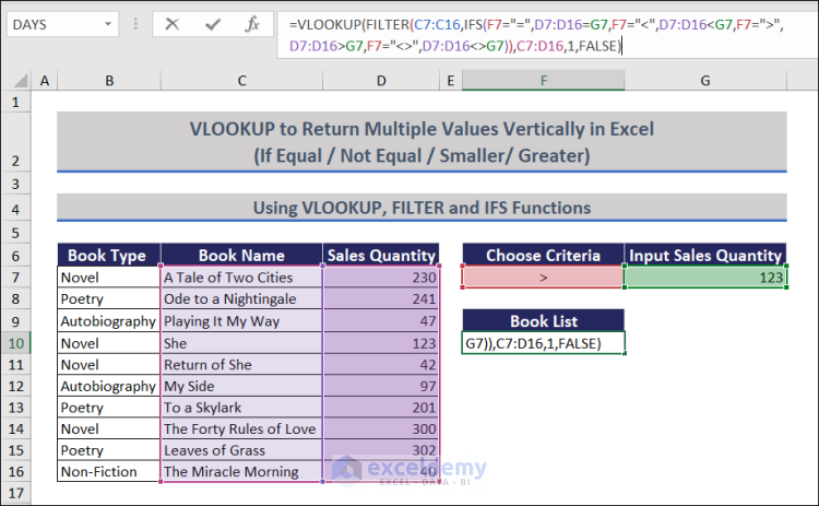
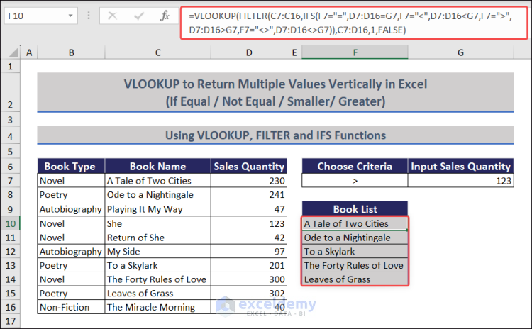
Step 4:
- Press Enter=> You will get multiple book names vertically for sales quantity greater than 123.
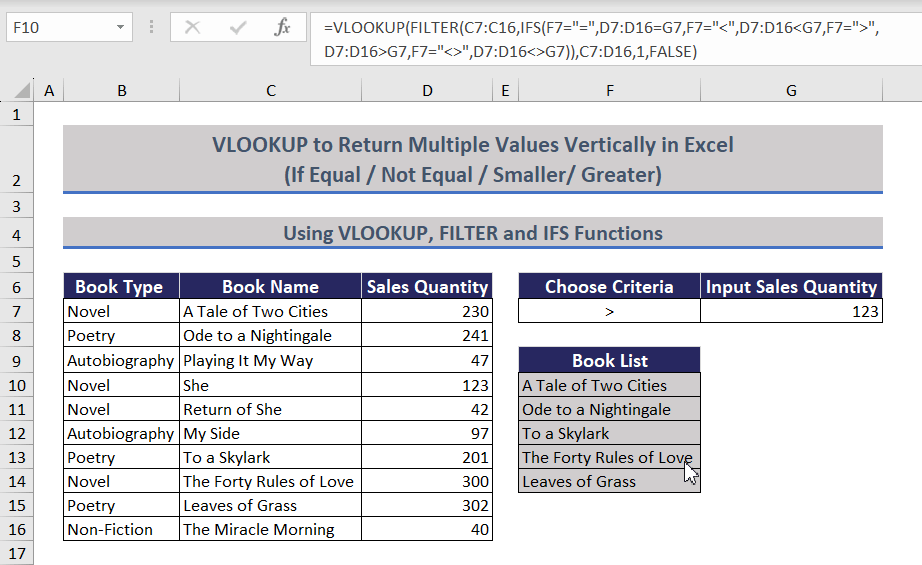
Step 5:
If you change the criteria in sales quantity, the VLOOKUP formula will return the book names vertically.
Observe the GIF.
Read More: VLOOKUP to Return Multiple Values Horizontally in Excel
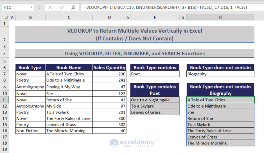
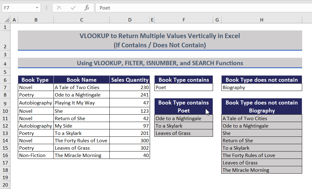
Method 3 – Combining the VLOOKUP, FILTER, ISNUMBER and SEARCH Functions to Return Multiple Values Vertically
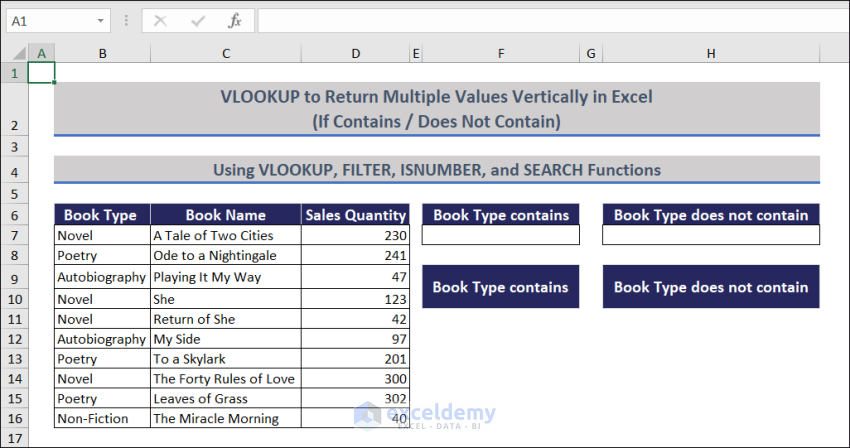
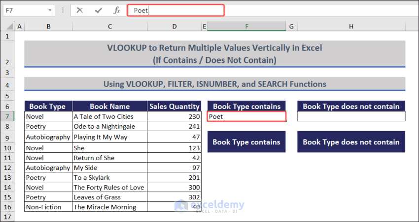
Step 1:
- Select F7 => Enter Poet.
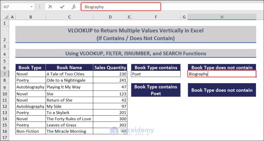
Step 2:
- Choose H7 => Enter Biography.
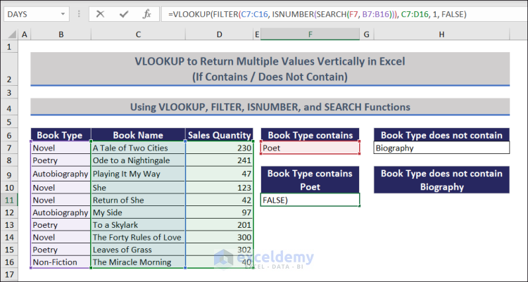
Step 3:
- Select F11 => Enter the following formula.
=VLOOKUP(FILTER(C7:C16, ISNUMBER(SEARCH(F7, B7:B16))), C7:D16, 1, FALSE)
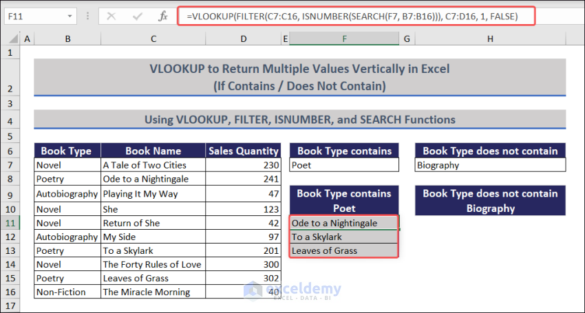
Step 4:
- Press Enter => You will see a list of book names that contain the text Poet.
Step 5:
- Select H11 =>Use the following formula.
=VLOOKUP(FILTER(C7:C16, ISNUMBER(SEARCH(H7, B7:B16))=FALSE), C7:D16, 1, FALSE)
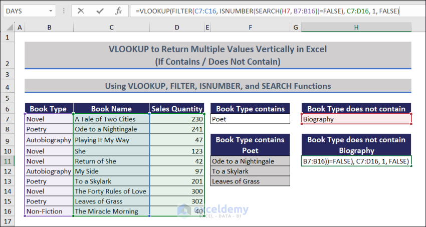
Step 6:
- Press Enter => You will see a list of book names that do not contain the word Biography.
Step 7:
If you change the words in F7 and H7, the formulas will return the book names vertically, as shown in the following GIF.
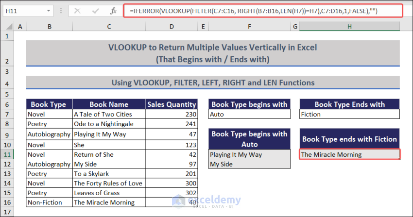
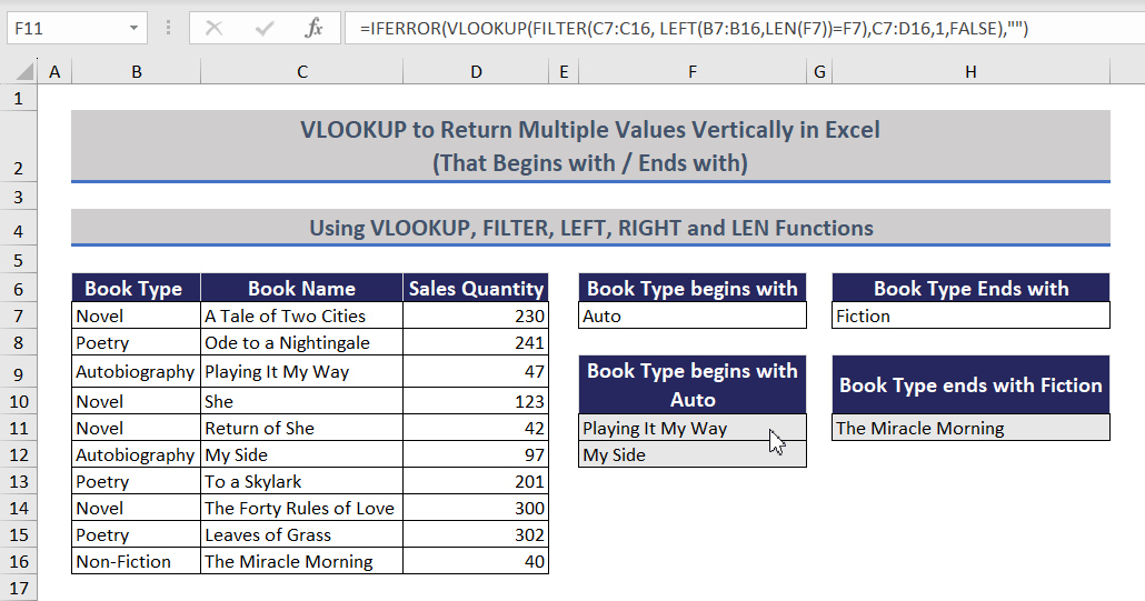
Method 4 – Using the VLOOKUP, FILTER, LEFT, and RIGHT Functions to Return Multiple Values Vertically
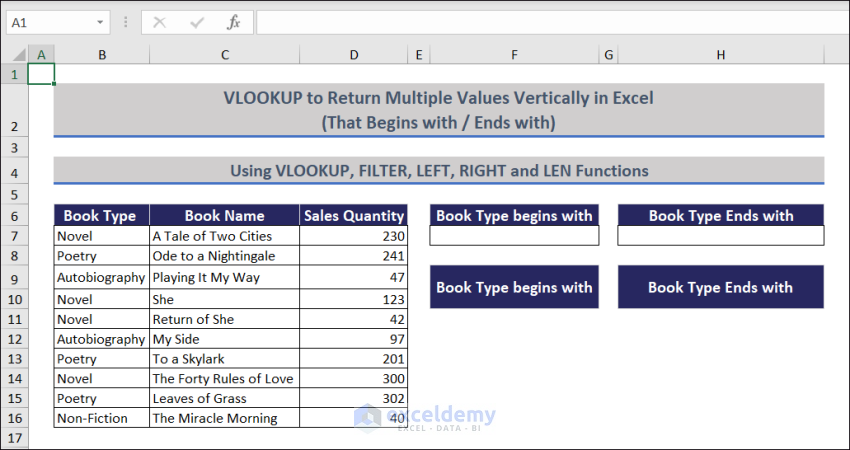
Step 1:
- Select F7 => Enter Auto.
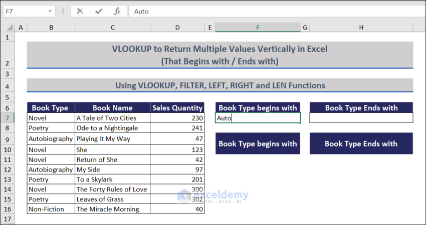
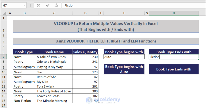
Step 2:
- Choose H7 => Enter Fiction.
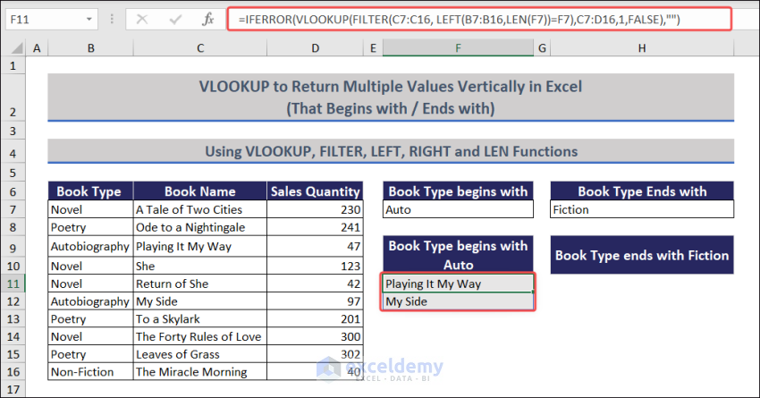
Step 3:
- Select F11 => use the following formula.
=IFERROR(VLOOKUP(FILTER(C7:C16, LEFT(B7:B16,LEN(F7))=F7),C7:D16,1,FALSE),"")
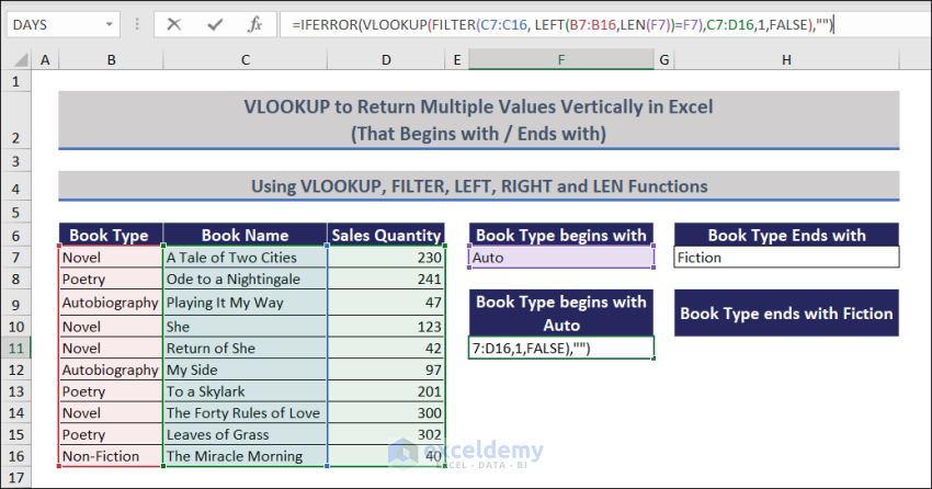
Step 4:
- Press Enter => You will see a list of book names that begin with the word Auto.
Step 5:
- Select H11 => Enter the following formula.
=IFERROR(VLOOKUP(FILTER(C7:C16,RIGHT(B7:B16,LEN(H7))=H7),C7:D16,1,FALSE),"")
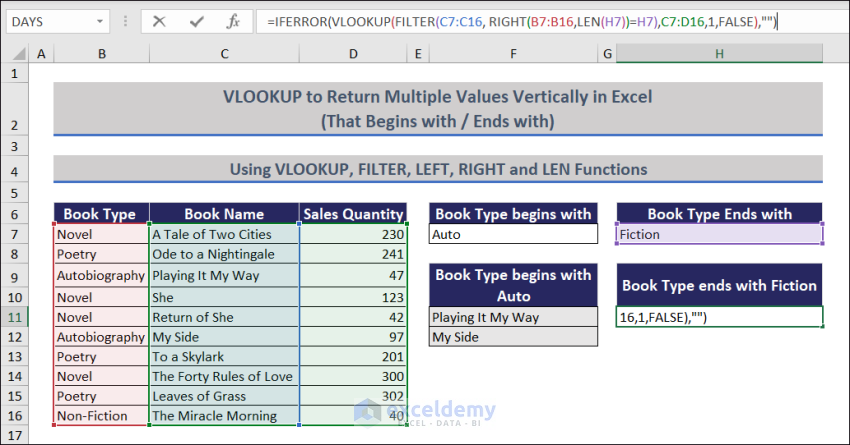
Step 6:
- Press Enter => You will see a list of book names ending with Fiction.
Step 7:
If you change the words in F7 and H7, the formulas will return the book names vertically, as shown in the following GIF.
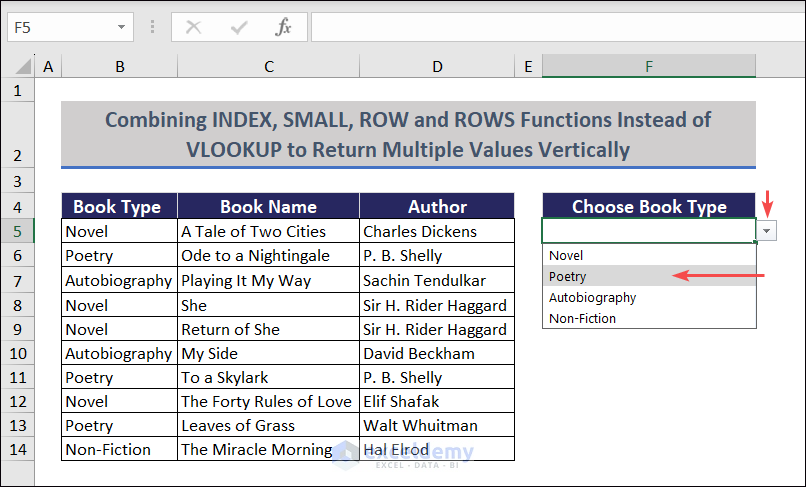
Method 5 – Using the INDEX, SMALL, ROW and ROWS Functions Instead of the VLOOKUP to Return Multiple Values Vertically
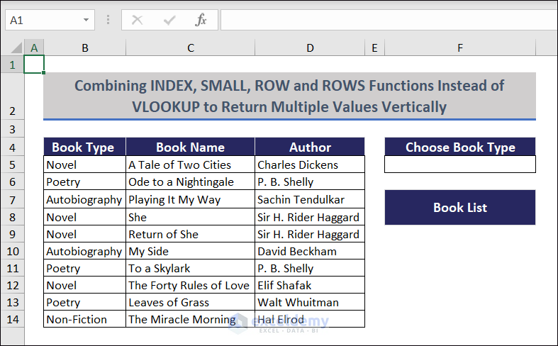
Step 1:
- Select F5 => Create a drop-down => Expand the drop-down => Choose Poetry.
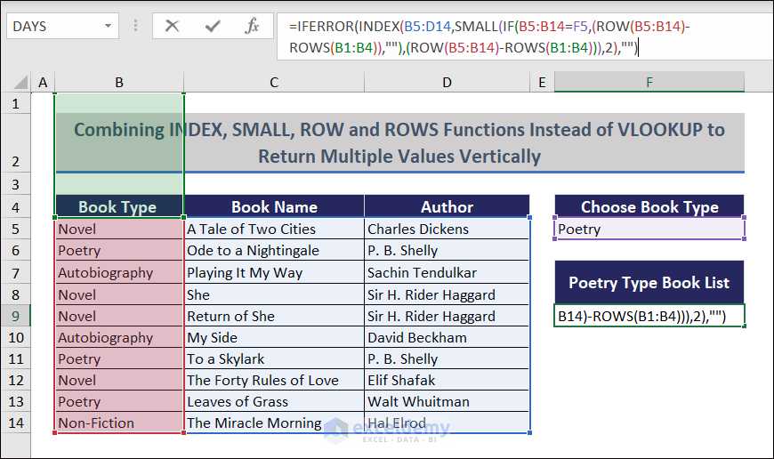
Step 2:
- Select F9 => Enter the following formula.
=IFERROR(INDEX(B5:D14,SMALL(IF(B5:B14=F5,(ROW(B5:B14)-ROWS(B1:B4)),""),(ROW(B5:B14)-ROWS(B1:B4))),2),"")
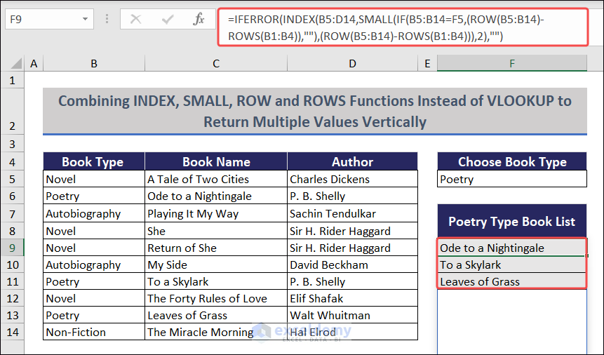
Step 3:
- Press Enter => You will see a list of poetry book names.
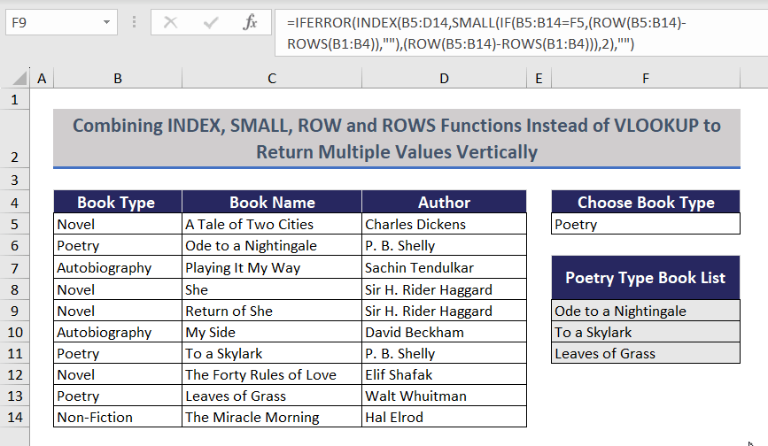
Step 4:
If you change the book type in F5, the formula will return the book names vertically, as shown in the following GIF.
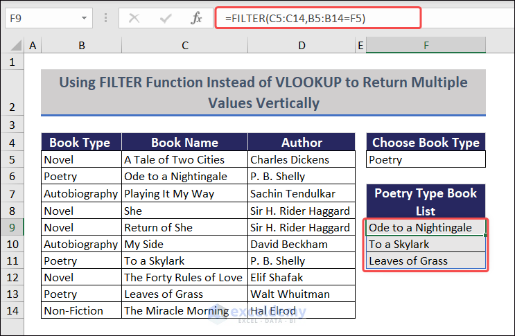
You can also use the FILTER function to return multiple values vertically.
=FILTER(C5:C14,B5:B14=F5)
Read More: How to Use VLOOKUP Function on Multiple Rows in Excel
Download Practice Workbook
Related Readings
- How to VLOOKUP Multiple Values in One Cell in Excel
- Excel VLOOKUP to Return Multiple Values in One Cell Separated by Comma
- Find Max of Multiple Values by Using VLOOKUP Function in Excel
<< Go Back to VLOOKUP Multiple Values | Excel VLOOKUP Function | Excel Functions | Learn Excel
Get FREE Advanced Excel Exercises with Solutions!

In you example, if the helper column only contains one value rather than multiples, it fills the entire search column with the same find. Any ideas as to how to fix this.
Go to the tab “When a criteria matches” and select ‘Non-Fiction’ to see what I mean. When there are multiple helpers for the book name it works fine.