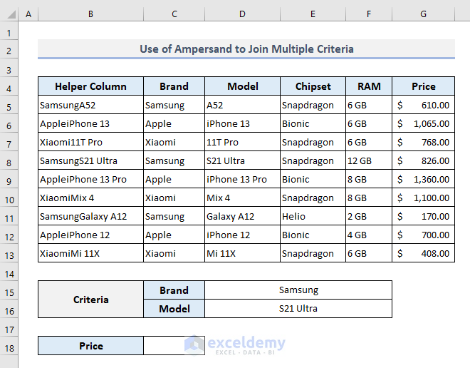
Example 1 – Using the Ampersand to Join Multiple Conditions in VLOOKUP in Excel
We have a dataset of smartphone models of three popular brands. Column B represents a helper column which is the combination of the values from Column C and Column D. This is because VLOOKUP only searches in the first column of a lookup table. We’ll fetch the price of the Samsung S21 Ultra.
- In the output Cell C18, the required formula will be:
=VLOOKUP(D15&D16,B5:G13,6,FALSE)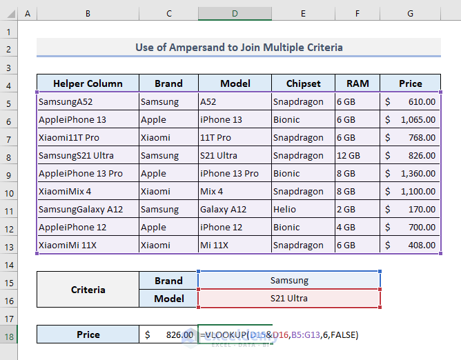
Example 2 – Combining VLOOKUP with the CHOOSE Function to Join Multiple Conditions in Excel
The CHOOSE function chooses a value or action to perform from a list of values based on its index number. The generic formula of this CHOOSE function is:
=CHOOSE(index_num, value1, [value2],…)
We’ll fetch the price of Samsung S21 Ultra from the table.
- The required formula in Cell C18 will be:
=VLOOKUP($D$15&$D$16,CHOOSE({1,2},$B$5:$B$13&$C$5:$C$13,$F$5:$F$13),2,FALSE)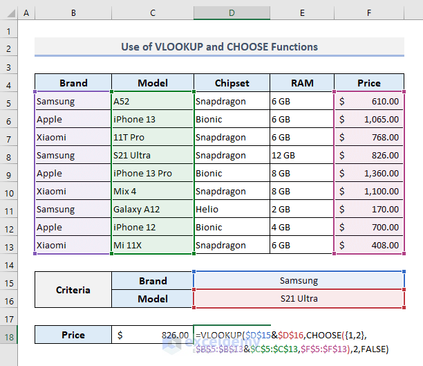
In this formula, CHOOSE function forms a table with Columns B, C, and F. As Columns B and C have been merged inside the CHOOSE function, they will represent a single column for the VLOOKUP function.
Read More: Vlookup with Multiple Criteria without a Helper Column in Excel
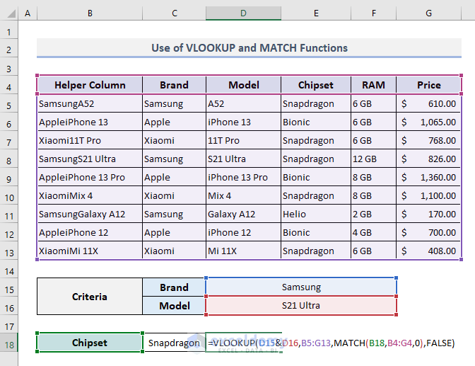
Example 3 – Joining VLOOKUP with the MATCH Function to Include Multiple Criteria in Excel
We’re back to the sample dataset with the helper column B.
- The required formula in Cell C18 will be:
=VLOOKUP(D15&D16,B5:G13,MATCH(B18,B4:G4,0),FALSE)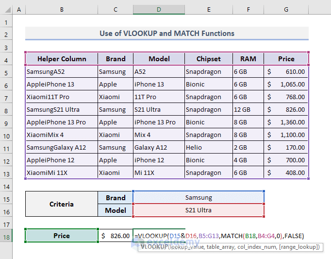
The MATCH function looks for the value present in Cell B18 in the array of B4:G4 and then returns the column number. This column number is then assigned to the third argument (col_num_index) of the VLOOKUP function.
If you change the output type in Cell B18, the corresponding result in Cell C18 will be updated. For example, if you type Chipset in Cell B18, the embedded formula in Cell C18 will show the chipset name for the specified smartphone model.
Read More: Use VLOOKUP with Multiple Criteria in Different Sheets
Example 4 – Combining VLOOKUP with the IF Function to Join Multiple Criteria
- The required formula in Cell C18 to pull out the price of the Samsung S21 Ultra will be:
=VLOOKUP(D15, IF(C5:C13=D16, B5:F13, ""), 5, FALSE)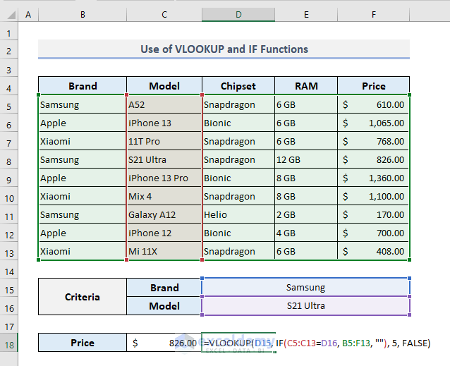
The IF function returns a partial array from B5:B13 depending on whether the corresponding value in column C matches the second criteria (D16). VLOOKUP then uses that partial array as its lookup table argument.
Example 5 – Using the VLOOKUP Function with Multiple Criteria in a Single Column in Excel
We want to get two smartphone models from Apple and Xiaomi.
- The required formula in the output Cell C18 should be:
=VLOOKUP(D15:D16,B5:F13,2,FALSE)
As the VLOOKUP function always extracts the first matched data, only the first model numbers of Apple and Xiaomi brands have appeared as return values.
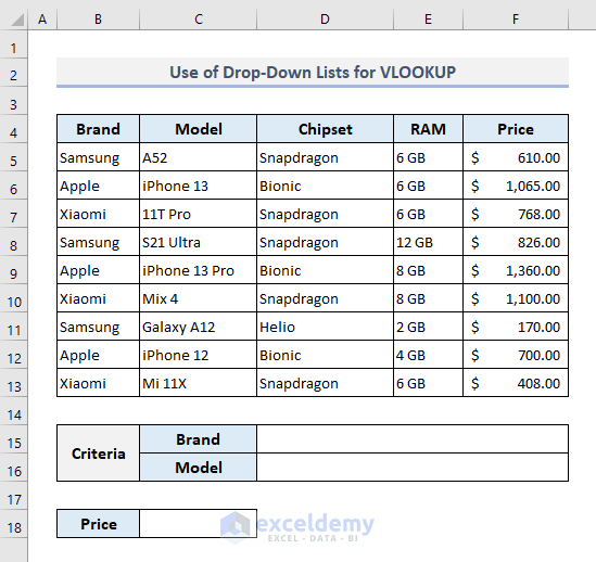
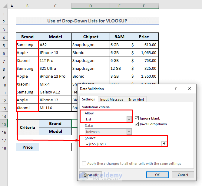
Example 6 – Using Drop-Down Lists as Multiple Criteria in VLOOKUP
We’ll create two drop-down lists for smartphone brands and model numbers in Cells D15 and D16.
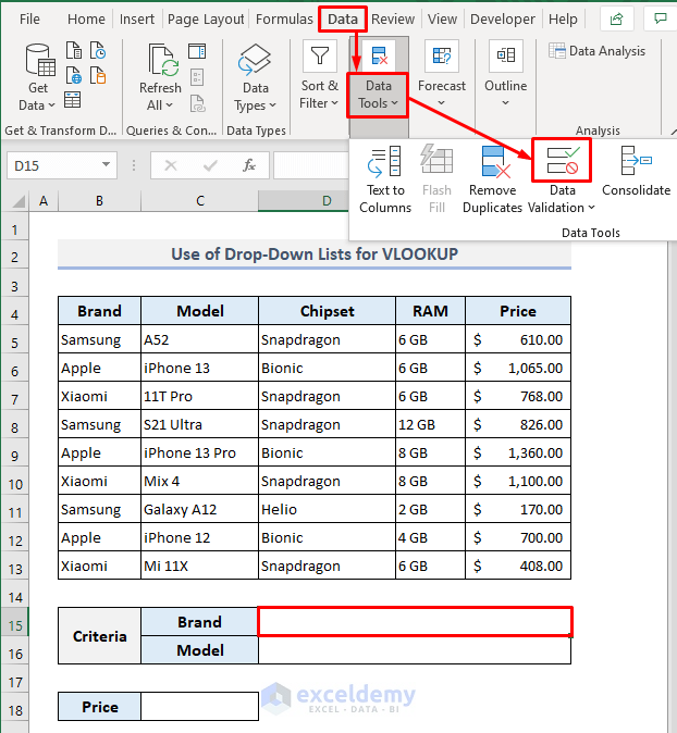
Step 1:
- Select Cell D15.
- In the Data tab, choose the Data Validation option from the Data Tools group.
- A dialog box will appear.
Step 2:
- In the Allow box, select the List option.
- Enable editing in the Source box and select the range of cells B5:B13.
- Press OK.
- The first drop-down list for the smartphone brands is now ready to use.
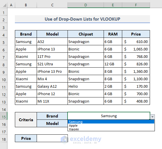
Step 3:
- Create another drop-down list for the smartphone model numbers. Select the range of cells C5:C13 in the Source option of the Data Validation dialog box here.
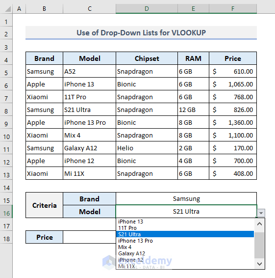
Step 4:
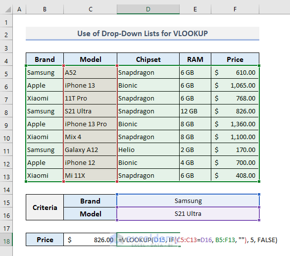
- In Cell 18, enter the following formula:
=VLOOKUP(D15, IF(C5:C13=D16, B5:F13, ""), 5, FALSE)- From the drop-down list, choose a smartphone brand and its model number, and you’ll be shown the price of the selected smartphone model.
- Every time you select a new smartphone brand and its model from the drop-down lists, the output cell with the price will get updated.
- If you select a combination that doesn’t exist, you’ll get an error.
Read More: Excel VLOOKUP with Multiple Criteria in Column and Row
Download the Practice Workbook
VLOOKUP with Multiple Criteria: Knowledge Hub
- VLOOKUP with Multiple Criteria and Multiple Results
- VLOOKUP with Multiple Criteria in Horizontal & Vertical Way
- Apply VLOOKUP with Multiple Criteria Using the CHOOSE Function
- VLOOKUP with Multiple Criteria Including Date Range in Excel
<< Go Back to Excel VLOOKUP Function | Excel Functions | Learn Excel
Get FREE Advanced Excel Exercises with Solutions!

Can I use lookup to populate the cells of one spreadsheet with the information from another using two separate criteria(date and text). I’ve tried using Vlookup but I keep having issues with the date. Google sheets keep misinterpreting it.
Hello, TEMITOPE!
You have asked a nice thing. Using VLOOKUP with dates is a complex thing sometimes and may result in errors easily. In this regard, you need to use the TEXT function.
Suppose, you have 5 columns in your table. You want the fifth column value for the C16 text and C15 date value. The date column is in the C5:C13 cells. In this situation, you can use the following formula for using VLOOKUP with text and date.
=VLOOKUP(C16,IF(TEXT(C5:C13,"mm/dd/yy")=TEXT(C15,"mm/dd/yy"), B5:F13, ""), 5, FALSE)Thank you for your query. We appreciate it so much.
Regards,
Tanjim Reza
Hello,
We have to lookup a percentage in a table, corresponding with a year.
Then we have then to multiply a value with this percentage.
We have to do this until the current year.
Can we use vlookup with a multiplication?
Hello, W BREKVELD!
Thank you for your query.
Yes, you can multiply a value with the looked-up percentage corresponding with a year. Just use the VLOOKUP function properly. Then write your desired multiplier in the formula bar before the used VLOOKUP function and then insert an asterisk (*) symbol.
Thus, the value will be multiplied by the looked-up percentage. And, to do this until the current year, use your fill handle feature to copy the same formula.
Regards,
Tanjim Reza