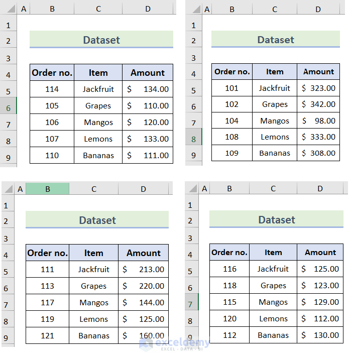
The sample dataset is an overview.
Method 1 – Using in VLOOKUP Function on Each Sheet Individually
Steps:
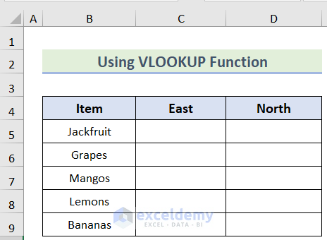
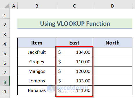
- Create a dataset as shown below.
- Enter the following formula in C5.
=VLOOKUP(B5, East!$C$5:$D$9, 2, FALSE)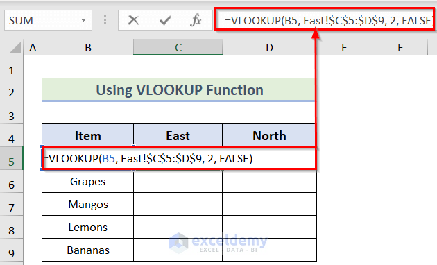
- Press Enter.
- Drag down the Fill Handle to see the result in the rest of the cells.
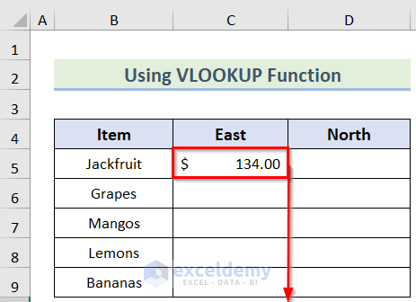
You will see the result in column C.
- Repeat the steps to see the result.

Read More: VLOOKUP with Multiple Criteria and Multiple Results
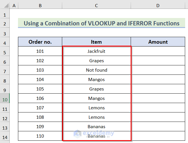
Method 2 – Using a Combination of the VLOOKUP and the IFERROR Functions
Steps:
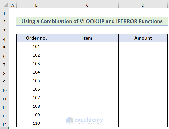
- Create a dataset as shown below.
- Enter the following formula in C5.
=IFERROR(VLOOKUP($B5, East!$B$5:$D$9, COLUMNS($B$4:C$4), FALSE), IFERROR(VLOOKUP($B5, West!$B$5:$D$9, COLUMNS($B$4:C$4), FALSE), "Not found"))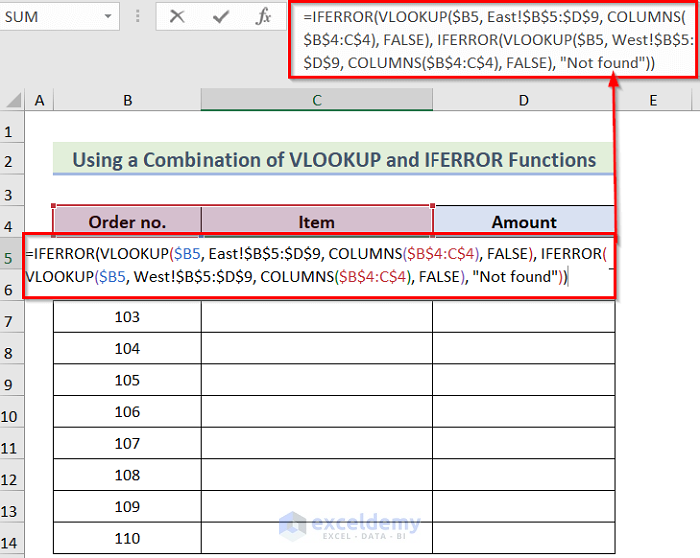
- Press Enter.
- Drag down the Fill Handle to see the result in the rest of the cells.
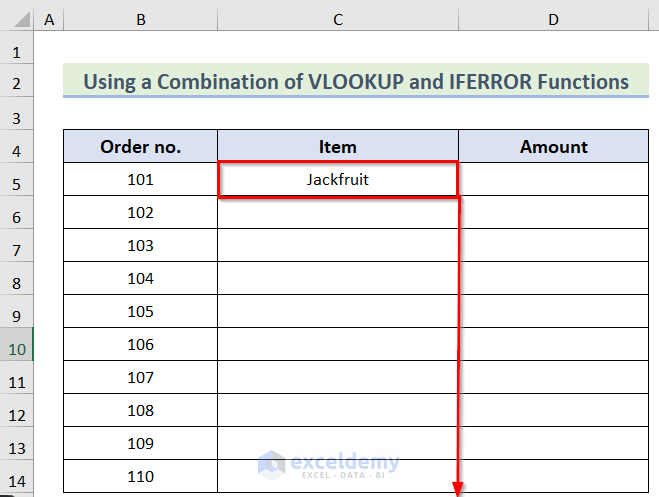
You will see the result in column C.
- Enter the following formula in D5.
=IFERROR(VLOOKUP($B5, East!$B$5:$D$9, COLUMNS($B$4:D$4), FALSE), IFERROR(VLOOKUP($B5, West!$B$5:$D$9, COLUMNS($B$4:D$4), FALSE), "Not found"))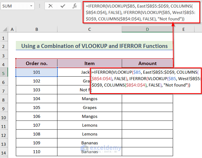
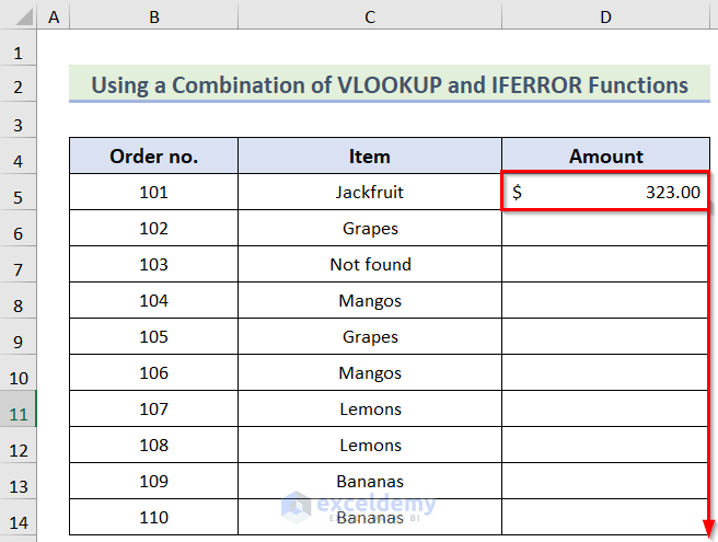
- Press Enter.
- Drag down the Fill Handle to see the result in the rest of the cells.
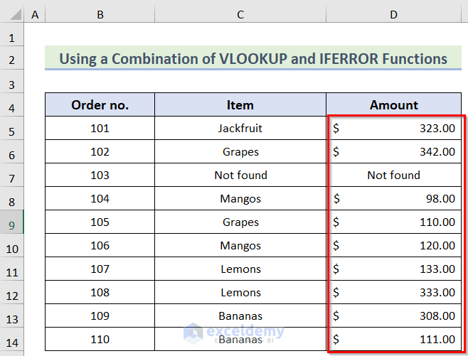
This is the output.
Formula Breakdown
- VLOOKUP($B5, West!$B$5:$D$9, COLUMNS($B$4:C$4), FALSE): finds the cell range you want to use.
- IFERROR(VLOOKUP($B5, East!$B$5:$D$9, COLUMNS($B$4:C$4), FALSE), IFERROR(VLOOKUP($B5, West!$B$5:$D$9, COLUMNS($B$4:C$4), FALSE), “Not found”)): applies the criteria in the formula.
Method 3 – Using a Combination of the VLOOKUP and Nested IFs Functions
Steps:
- Enter the following formula in C5.
=VLOOKUP($B5, IF(C$4="east", East_sales, IF(C$4="north", North_sales, IF(C$4="south", South_sales, IF(C$4="west", West_sales)))), 2, FALSE)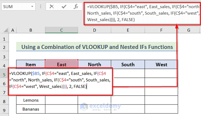
- Press Enter.
- Drag down the Fill Handle to see the result in the rest of the cells.
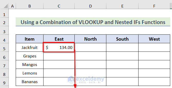
You will see the result in column C.
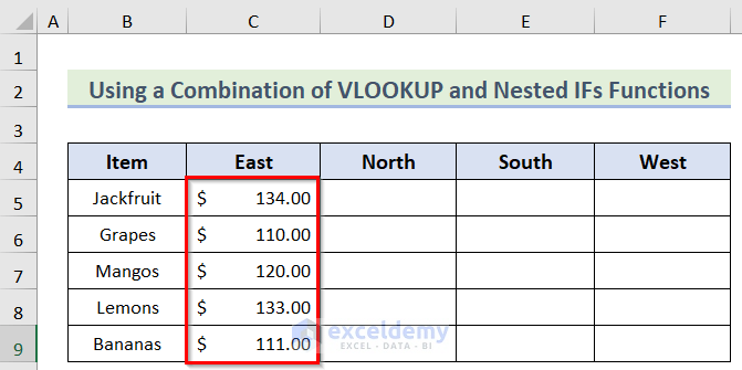
- This is the output.

Formula Breakdown
- IF(C$4=” west”, West_sales): represents the selected sheets you want to use.
- VLOOKUP($B5, IF(C$4=”east”, East_sales, IF(C$4=”north”, North_sales, IF(C$4=”south”, South_sales, IF(C$4=”west”, West_sales)))), 2, FALSE): represents the conditions in the selected sheets.
Read More: Vlookup with Multiple Criteria without a Helper Column in Excel
Method 4 – Combining the VLOOKUP and the INDIRECT Functions
Steps:
- Enter the following formula in C5.
=VLOOKUP($B5, INDIRECT(C$4&"_sales"), 2, FALSE)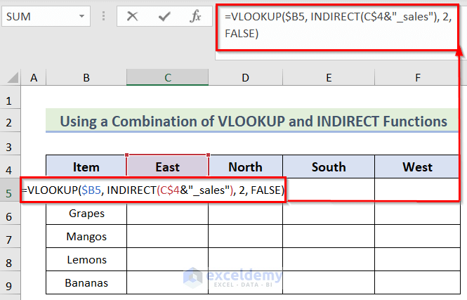
- Press Enter.
- Drag down the Fill Handle to see the result in the rest of the cells.
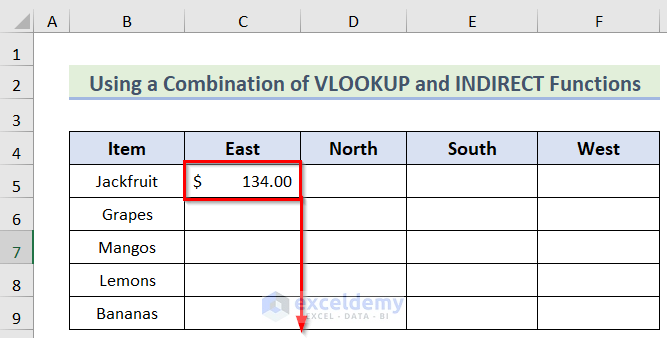
You will see the result in column C.
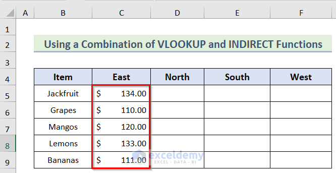
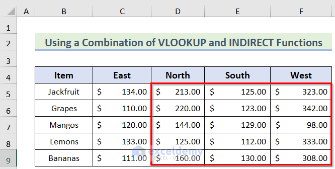
This is the output.
Formula Breakdown
- INDIRECT(C$4&”_sales”): represents the selected sheets.
- VLOOKUP($B5, INDIRECT(C$4&”_sales”), 2, FALSE): takes the search value and finds the result according to the condition.
Read More:How to Apply VLOOKUP with Multiple Criteria Using the CHOOSE Function
How to Use the VLOOKUP with Multiple Matches
Steps:
- Enter the following formula in B5.
=C5&COUNTIF(C5:$C$10,C5)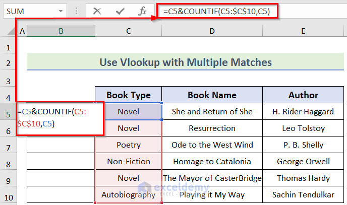
- Press Enter.
- Drag down the Fill Handle to see the result in the rest of the cells.
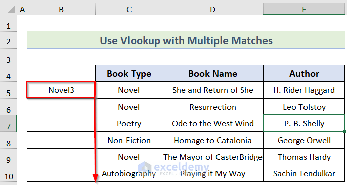
You will see the result in column B.

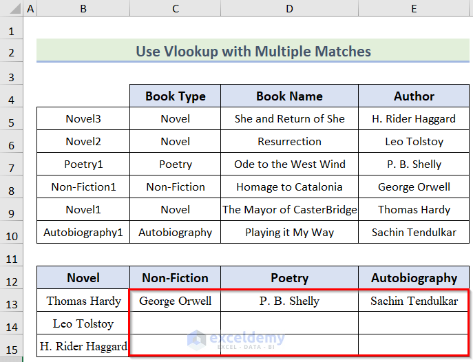
- Enter the following formula in B13.
=VLOOKUP(B$12&ROW($A$1:INDIRECT("A"&COUNTIF($C$5:$C$10,B$12))),$B$5:$E$10,4,FALSE)
You will see the result in column B.

This is the output.
Formula Breakdown
- COUNTIF($C$5:$C$10, B$12): represents the selected cells.
- INDIRECT(“A”&COUNTIF($C$5:$C$10,B$12)): applies the conditions.
- VLOOKUP(B$12&ROW($A$1:INDIRECT(“A”&COUNTIF($C$5:$C$10, B$12))),$B$5:$E$10,4, FALSE): takes the values and finds the result according to the criteria.
Read More: VLOOKUP with Multiple Criteria Including Date Range in Excel
Download Practice Workbook
Download the practice workbook.
Related Articles
- Excel VLOOKUP with Multiple Criteria in Horizontal & Vertical Way
- Excel VLOOKUP with Multiple Criteria in Column and Row
<< Go Back to VLOOKUP with Multiple Criteria | Excel VLOOKUP Function | Excel Functions | Learn Excel
Get FREE Advanced Excel Exercises with Solutions!
