While working in Excel, we often need to find a value by applying the VLOOKUP function with multiple criteria using the CHOOSE function. VLOOKUP function is one of the most used functions of Excel. Basically, the VLOOKUP function doesn’t deal with multiple criteria unless we make any change within formula e.g. adding ampersand operator. But by combining the VLOOKUP function with the CHOOSE function, we can use VLOOKUP function with multiple criteria in a more sophisticated way.
How to Apply VLOOKUP with Multiple Criteria Using the CHOOSE Function: 2 Easy Steps
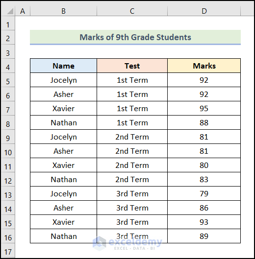
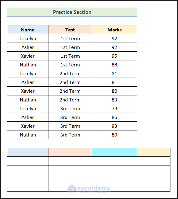
In this section of the article, we will learn 2 simple methods to apply the VLOOKUP function with multiple criteria using theCHOOSE function. Let’s say, we have Marks of 9th Grade Students as our dataset. In the dataset, we have the Marks of the students for their 3 Tests. We will extract the Marks of the students depending on their Name and Test by using a combination of VLOOKUP and CHOOSE functions. Let’s follow the steps mentioned below to do this.
Not to mention that we have used the Microsoft Excel 365 version for this article, you can use any other version according to your convenience
Step 01: Create Output Table
In the first step, we will create our output table to display our extracted outputs. To do this, we will use the UNIQUE and the TRANSPOSE function of Excel. The UNIQUE function returns a set of unique cells from an array of cells. The TRANSPOSE function converts the columns into rows while keeping the data intact. Let’s use the procedure discussed in the following section.
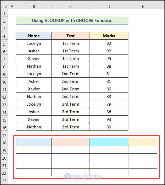
- Firstly, create a blank table as shown in the following image.
- After that, enter the following formula in cell B18.
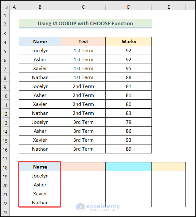
=UNIQUE(B4:B16)Here, the range of cell B4:B16 indicates the cells of the Name column. Now, the formula will return a set of unique values from the cell range B4:B16.
- Following that, press ENTER.

Consequently, you will have the unique values from the Name column as marked in the following picture.
- After that, use the following formula in cell C18.
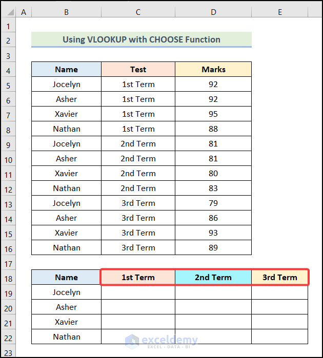
=TRANSPOSE(UNIQUE(C5:C16))Here, the range of cells C5:C16 refers to the cells of the Test column. Now, the formula will return a transposed set of unique values from the cell range C5:C16.
- Then, hit ENTER.

As a result, you will have the Test names in rows as shown in the image below.
Step 02: Use VLOOKUP Function with CHOOSE Function
Now, we will use the VLOOKUP and CHOOSE functions of Excel to extract output depending on multiple criteria. Let’s use the steps given below to do this.
- Firstly, enter the formula given below in cell C19.
=VLOOKUP($B19&"|"&C$18,CHOOSE({1,2},$B$5:$B$16&"|"&$C$5:$C$16,$D$5:$D$16),2,0)Here, cell B19 indicates a cell of the Name column, cell C18 refers to the 1st cell of the transposed row of the output table, and the range $D$5:$D$16 represents the cells of the Marks column of the dataset.
Formula Breakdown
- CHOOSE({1,2},$B$5:$B$16&”|”&$C$5:$C$16,$D$5:$D$16) → It returns a value from a range of values depending on the index number.
- {1,2} → This is the index_num argument.
- $B$5:$B$16&”|”&$C$5:$C$16 → It refers to the value1 argument.
- $D$5:$D$16 → It is the value2 argument.
- Output → {“Jocelyn|1st Term”,92;”Asher|1st Term”,92;”Xavier|1st Term”,95;”Nathan|1st Term”,88;”Jocelyn|2nd Term”,81;”Asher|2nd Term”,81;”Xavier|2nd Term”,80;”Nathan|2nd Term”,83;”Jocelyn|3rd Term”,79;”Asher|3rd Term”,86;”Xavier|3rd Term”,93;”Nathan|3rd Term”,89}.
- This is the table_array of the VLOOKUP function.
- Now, in the VLOOKUP function,
- $B19&”|”&C$18 → This is the lookup_value argument.
- CHOOSE({1,2},$B$5:$B$16&”|”&$C$5:$C$16,$D$5:$D$16) → It refers to the table_array argument.
- 2 → It indicates the col_index_num argument.
- 0 → This represents the [range_lookup] argument.
- Output → 92.
- Now, press ENTER.

Consequently, you will have the following output on your worksheet.

- After that, drag the Fill Handle along the row up to cell E19 and you will have the Marks of Jocelyn in her 3 Tests.

- Next, use the AutoFill feature of Excel to obtain the remaining outputs as shown in the following picture.

How to Use VLOOKUP Function with Multiple Criteria in Different Sheets
While working in Excel, we often use the VLOOKUP function with multiple criteria. For the large dataset and the output table, it becomes difficult to accommodate both the dataset and the output table in a single worksheet. So, in those situations, we use separate sheets for the dataset and the output table. Let’s use the steps discussed in the following section to do this.
Step 01: Create Output Table
In the beginning, we will create our output table to show the outputs. To do this, again we will use the UNIQUE and the TRANSPOSE functions of Excel. Let’s follow the steps below.
- Firstly, create a blank table as shown in the following image.
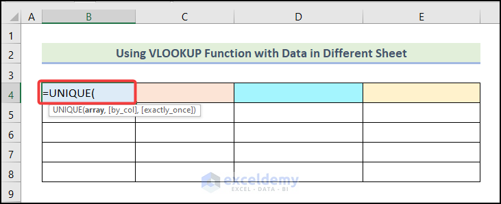
- Following that, type in the following formula in cell B4.
=UNIQUE(Note: This is not the complete formula. The formula will be completed when we will close the parentheses.
- After that, go to the worksheet named Dataset and select the cells of the Name column along with the column header.
- Then, close the parentheses.

- Now, as our formula is completed, press ENTER.
=UNIQUE(Dataset!B4:B16)Consequently, you will have the following output on your worksheet.

- Next, type in the following formula in cell C4.
=TRANSPOSE(UNIQUE(
- After that, go to the Dataset worksheet and select the cells under the Test column as marked in the following image.
- Now, close the parentheses of the 2 functions.

- Finally, as the formula is completed now, hit ENTER.
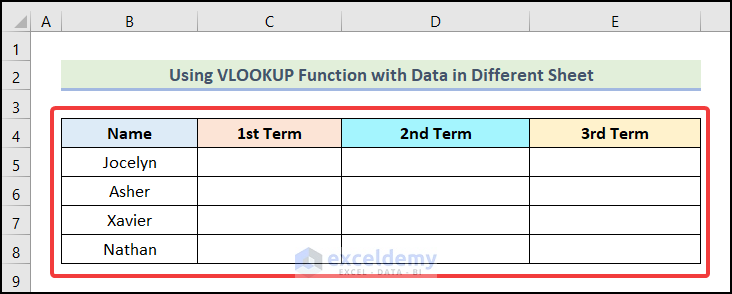
=TRANSPOSE(UNIQUE(Dataset!C5:C16))As a result, your output table will be ready and it will look like the following image.
Step 02: Apply VLOOKUP Function
In this step, we will apply the VLOOKUP function to extract output from a different worksheet.
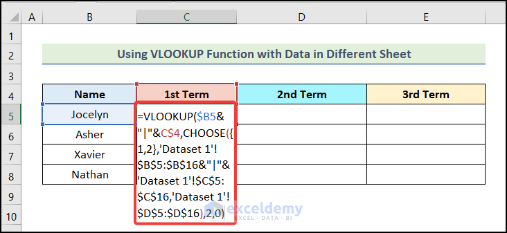
- Firstly, enter the following formula in cell C5.
=VLOOKUP($B5&"|"&C$4,CHOOSE({1,2},Dataset!$B$5:$B$16&"|"&Dataset!$C$5:$C$16,Dataset!$D$5:$D$16),2,0)Formula Breakdown
- CHOOSE({1,2},Dataset!$B$5:$B$16&”|”&Dataset!$C$5:$C$16,Dataset!$D$5:$D$16) → It gives us value from a range of values depending on the index number.
- {1,2} → This is the index_num argument.
- Dataset!$B$5:$B$16&”|”&Dataset!$C$5:$C$16 → It represents the value1 argument.
- Dataset!$D$5:$D$16 → It is the value2 argument.
- Output → {“Jocelyn|1st Term”,92;”Asher|1st Term”,92;”Xavier|1st Term”,95;”Nathan|1st Term”,88;”Jocelyn|2nd Term”,81;”Asher|2nd Term”,81;”Xavier|2nd Term”,80;”Nathan|2nd Term”,83;”Jocelyn|3rd Term”,79;”Asher|3rd Term”,86;”Xavier|3rd Term”,93;”Nathan|3rd Term”,89}
- This is the table_array of the VLOOKUP function.
- Now, in the VLOOKUP function,
- $B5&”|”&C$4 → This is the lookup_value argument.
- CHOOSE({1,2},Dataset!$B$5:$B$16&”|”&Dataset!$C$5:$C$16,Dataset!$D$5:$D$16) → It refers to the table_array argument.
- 2 → It indicates the col_index_num argument.
- 0 → This represents the [range_lookup] argument.
- Output → 92.
- Following that, press ENTER.
Consequently, you will have the following output on your worksheet.

- Now, drag the Fill Handle in the row direction up to cell E5 and you will have the Marks of Jocelyn for her 3 Tests.

- Finally, by using the AutoFill option of Excel, you will get the rest of the outputs as demonstrated in the following image.

Read More: How to Use VLOOKUP with Multiple Criteria in Different Sheets
Practice Section
In the Excel Workbook, we have provided a Practice Section on the right side of the worksheet. Please practice it by yourself.
Download Practice Workbook
Conclusion
That’s all about today’s session. I strongly believe that this article was able to guide you to VLOOKUP with Multiple Criteria Using the CHOOSE Function. Please feel free to leave a comment if you have any queries or recommendations for improving the article’s quality.
Related Articles
- Excel VLOOKUP with Multiple Criteria in Column and Row
- VLOOKUP with Multiple Criteria and Multiple Results
- How to Use VLOOKUP with Multiple Criteria in Different Columns
- Excel VLOOKUP with Multiple Criteria in Horizontal & Vertical Way
- VLOOKUP with Multiple Criteria Including Date Range in Excel
- Vlookup with Multiple Criteria without a Helper Column in Excel
<< Go Back to VLOOKUP with Multiple Criteria | Excel VLOOKUP Function | Excel Functions | Learn Excel
Get FREE Advanced Excel Exercises with Solutions!
