VLOOKUP with Multiple Criteria and Multiple Results (8 Examples)

If you are looking for a way to use the VLOOKUP function with multiple criteria and multiple results, then this article will be helpful for you. The main focus of this article is to explain how you can use VLOOKUP with multiple criteria and multiple results in Excel.

How to Use VLOOKUP with Multiple Criteria and Multiple Results: 8 Suitable Examples

Here, I have taken the following dataset to explain this article. This dataset contains the Sales Overview of some Products for the months of January, February, and March. I will look up values with multiple criteria and then return multiple results that match those criteria. I will explain 8 different examples of using VLOOKUP with multiple criteria and multiple results.

1. Using Ampersand Operator to VLOOKUP with Multiple Criteria

In this first example, I will show you how you can use Ampersand Operator (&) to use VLOOKUP with multiple criteria and return multiple results. For this example, I have taken the following dataset. Suppose, you want to find the Sales of Headphones in the State of Florida. I will show you how you can find Sales for the months of January, February, and March.

Let’s see the steps.

Steps:

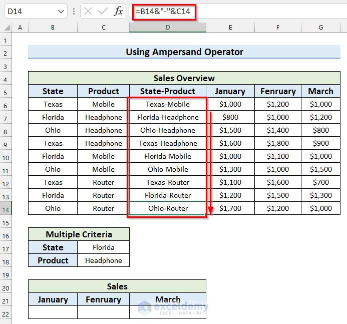
Firstly, create a column to represent both criteria in the same column. Here, I created mine and named it State-Product.

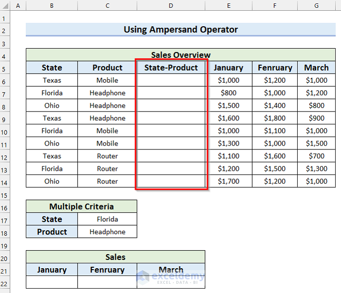
Secondly, select the first cell of the column you created. Here, I selected cell D6.
Thirdly, in cell D6 write the following formula.

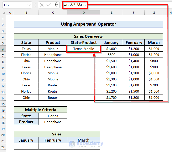
=B6&"-"&C6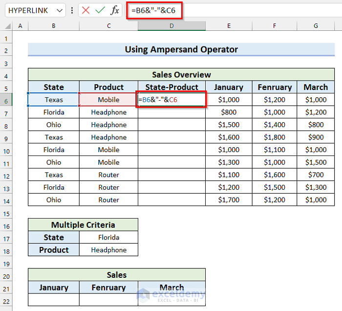

Here, the Ampersand Operator will join the texts and return the joined texts as result.

After that, press ENTER to get the result.

Then, drag the Fill Handle to copy the formula.

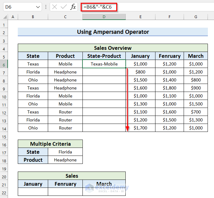
Finally, you can see that I have copied the formula to all the other cells and combined both of the criteria in the same column.

Now, I will use the VLOOKUP function to find the Sales for the months of January, February, and March.

Firstly, select the cell where you want to find the Sales for January. Here, I selected cell B22.
Secondly, in cell B22 write the following formula.

=VLOOKUP(C17&"-"&C18,D6:G14,{2,3,4},FALSE))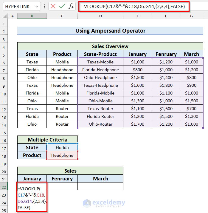

Formula Breakdown

C17&”-“&C18 —-> Here, the Ampersand Operator (&) will join the texts.
- Output: “Florida-Headphone”
VLOOKUP(C17&”-“&C18,D6:G14,{2,3,4},FALSE) —-> turns into
- VLOOKUP(“Florida-Headphone”,D6:G14,{2,3,4},FALSE) —-> Here, the VLOOKUP function will find the matches for the lookup_value from column 2, 3, and 4 and return the Sales as an array.
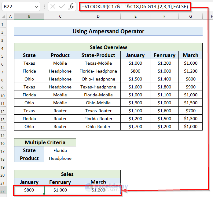
  - Output: {800,1000,1200}

Finally, press ENTER to get multiple results. If you are using an older version of Microsoft Excel than Excel 2019, then press CTRL+SHIFT+ENTER to get the results.

Note: In this case, you have to make sure that the lookup_value remains in the leftmost column of the table_array because that is where the function is going to look for the match.

2. Applying CONCATENATE Function to VLOOKUP with Multiple Criteria and Return Multiple Results

In this method, I will show you how you can use the CONCATENATE function to join the multiple criteria as lookup_value in the VLOOKUP function. Here, I have taken the same example as before. I will show you how you can find the Sales for a specific Product from a specific State and return multiple results.

Let’s see the steps.

Steps:

Firstly, create a column combining both criteria by following the steps from Example-01.

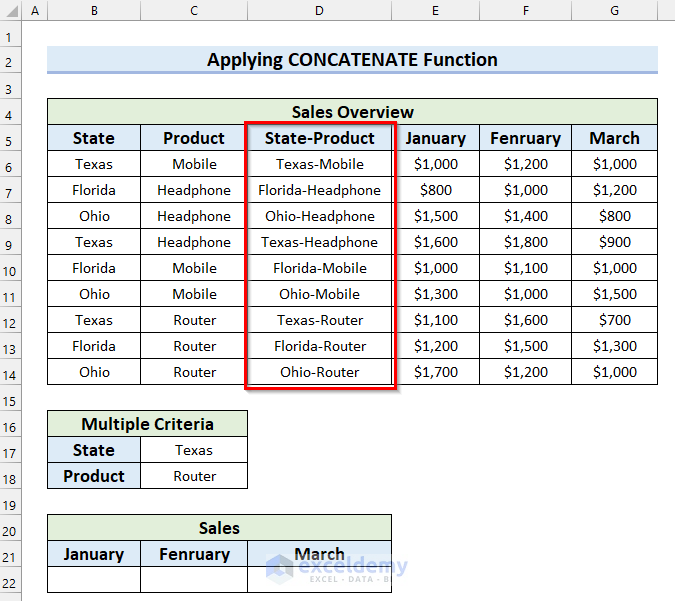
After that, select the cell where you want to find Sales for January. Here, I selected cell B22.
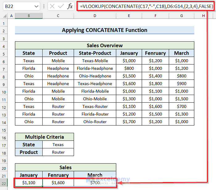
Then, in cell B22 write the following formula.

=VLOOKUP(CONCATENATE(C17,"-",C18),D6:G14,{2,3,4},FALSE)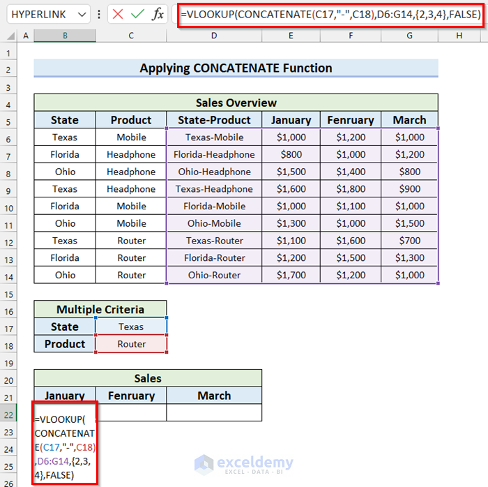

Formula Breakdown

CONCATENATE(C17,”-“,C18) —-> Here, the CONCATENATE function will combine the texts from cells C17 and C18.
- Output: “Texas-Router”
VLOOKUP(CONCATENATE(C17,”-“,C18),D6:G14,{2,3,4},FALSE) —-> turns into
- VLOOKUP(“Texas-Router”,D6:G14,{2,3,4},FALSE) —-> Now, the VLOOKUP function will find the matches for the lookup_value from columns 2, 3, and 4 and return the Sales as an array.
  - Output: {1100,1600,700}

Finally, press ENTER to get the results. If you are using an older version of Microsoft Excel than Excel 2019, then press CTRL+SHIFT+ENTER to get the results.

3. Employing CHOOSE Function to VLOOKUP with Multiple Criteria

In this example, I will show you how you can employ the CHOOSE function to use VLOOKUP with multiple criteria and get multiple results in Excel. Here, I have taken the following dataset for this example. Suppose you have a dataset containing State, Product, and Sales in the months of January and February. You want to find the Sales for both months for a specific Product in a specific State.

Let’s see how you can do it.

Steps:

Firstly, select the cell where you want to find the Sales for January. Here, I selected cell G10.
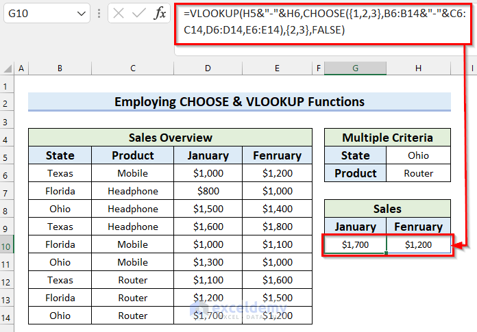
Secondly, in cell G10 write the following formula.

=VLOOKUP(H5&"-"&H6,CHOOSE({1,2,3},B6:B14&"-"&C6:C14,D6:D14,E6:E14),{2,3},FALSE)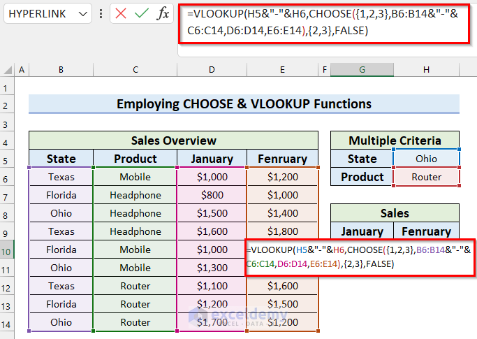

Formula Breakdown

H5&”-“&H6 —-> Here, the Ampersand Operator will join the texts.
- Output: “Ohio-Router”
B6:B14&”-“&C6:C14 —-> Now, the Ampersand Operator will join these 2 columns and return as 1 column.
- Output: {“Texas-Mobile”;”Florida-Headphone”;”Ohio-Headphone”;”Texas-Headphone”;”Florida-Mobile”;”Ohio-Mobile”;”Texas-Router”;”Florida-Router”;”Ohio-Router”}
CHOOSE({1,2,3},B6:B14&”-“&C6:C14,D6:D14,E6:E14) —-> turns into
- CHOOSE({1,2,3},{“Texas-Mobile”;”Florida-Headphone”;”Ohio-Headphone”;”Texas-Headphone”;”Florida-Mobile”;”Ohio-Mobile”;”Texas-Router”;”Florida-Router”;”Ohio-Router”},D6:D14,E6:E14) —-> Here, the CHOOSE function will return a table containing 3 columns.
  - Output: {“Texas-Mobile”,1000,1200;”Florida-Headphone”,800,1000;”Ohio-Headphone”,1500,1400;”Texas-Headphone”,1600,1800;”Florida-Mobile”,1000,1100;”Ohio-Mobile”,1300,1000;”Texas-Router”,1100,1600;”Florida-Router”,1200,1500;”Ohio-Router”,1700,1200}
VLOOKUP(H5&”-“&H6,CHOOSE({1,2,3},B6:B14&”-“&C6:C14,D6:D14,E6:E14),{2,3},FALSE) —-> turns into
- VLOOKUP(“Ohio-Router”,{“Texas-Mobile”,1000,1200;”Florida-Headphone”,800,1000;”Ohio-Headphone”,1500,1400;”Texas-Headphone”,1600,1800;”Florida-Mobile”,1000,1100;”Ohio-Mobile”,1300,1000;”Texas-Router”,1100,1600;”Florida-Router”,1200,1500;”Ohio-Router”,1700,1200},{2,3},FALSE) —-> Here, the VLOOKUP function will find the match for lookup_value from columns 2 and 3 and then return multiple results as array.
  - Output: {1700,1200}

Thirdly, press ENTER to get the results. If you are using an older version of Microsoft Excel than Excel 2019, then press CTRL+SHIFT+ENTER to get the results.

4. Using MAX and VLOOKUP Functions with Multiple Criteria to Return Multiple Results

In this example, I will show you how you can use the MAX function with VLOOKUP with multiple criteria and get multiple results. Here, I have taken the following dataset for this example. It contains Sales, State, and Product. Now, I will find which Product from which State has the Maximum Sales.

Let’s see the steps.

Steps:

First, select the cell from where you want your multiple results to start. Here, I selected cell F6.
Secondly, in cell F6 write the following formula.

=VLOOKUP(MAX(B6:B14),B6:D14,{2,3},FALSE)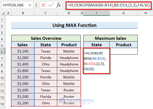

Formula Breakdown

MAX(B6:B14) —-> Here, the MAX function will return the largest value among the cell range B6:B14.
- Output: 1800
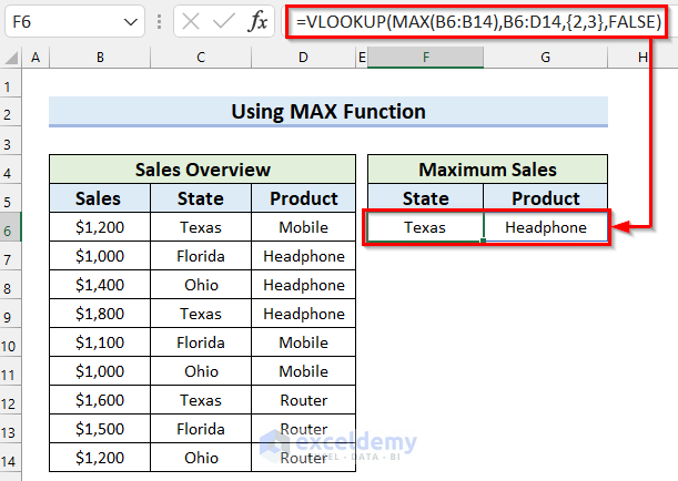
VLOOKUP(MAX(B6:B14),B6:D14,{2,3},FALSE) —-> turns into
- VLOOKUP(1800,B6:D14,{2,3},FALSE) —-> Here, the VLOOKUP function will look for match for lookup_value and return multiple results from columns 2 and 3 as an array.
  - Output: {“Texas”,”Headphone”}

After that, press ENTER to get the results. If you are using an older version of Microsoft Excel than Excel 2019, then press CTRL+SHIFT+ENTER to get the results.

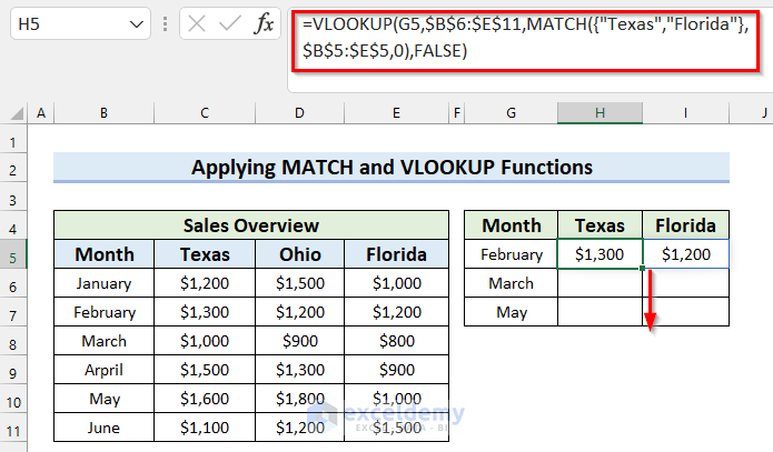
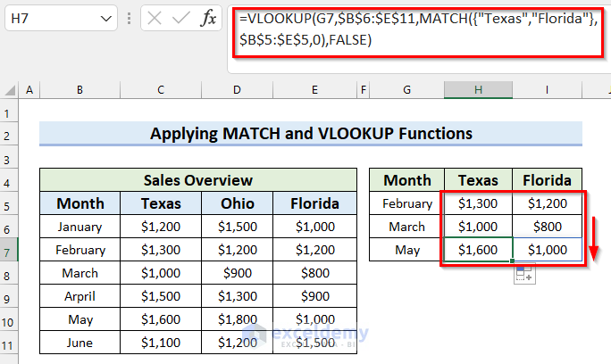
5. Applying MATCH and VLOOKUP Functions for Multiple Criteria

Here, I will show you how you can use the MATCH function and the VLOOKUP function together for multiple criteria and multiple results. For this example, I have taken the following dataset. It contains a Sales Overview for 6 Months for the States of Texas, Ohio, and Florida. Now, I will show you how you can find Sales for a specific Month for multiple States.

Let’s see the steps.

Steps:

Firstly, select the cell from where you want to start your multiple results. Here, I selected cell H5.
Secondly, in cell H5 write the following formula.

=VLOOKUP(G5,$B$6:$E$11,MATCH({"Texas","Florida"},$B$5:$E$5,0),FALSE)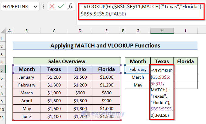

Formula Breakdown

MATCH({“Texas”,”Florida”},$B$5:$E$5,0) —-> Here, the MATCH function will return the relative position of the lookup_value in the lookup_array.
- Output: {2,4}
VLOOKUP(G5,$B$6:$E$11,MATCH({“Texas”,”Florida”},$B$5:$E$5,0),FALSE) —-> turns into
- VLOOKUP(G5,$B$6:$E$11,{2,4},FALSE) —-> Here, the VLOOKUP function will look for a match for the lookup_value and return multiple results from columns 2 and 4 as an array.
  - Output: {1300,1200}

Thirdly, press ENTER to get the results. If you are using an older version of Microsoft Excel than Excel 2019, then press CTRL+SHIFT+ENTER to get the results.

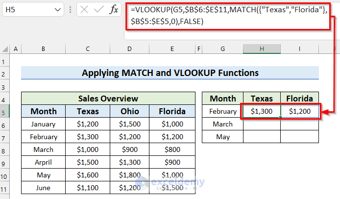
After that, drag the Fill Handle to get the result.

Finally, you can see that I have copied the formula to the other cells and got multiple results.

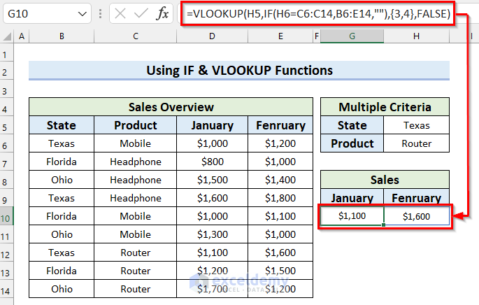
6. Using IF & VLOOKUP Functions with Multiple Criteria and Multiple Results

In this example, I will explain how you can use the IF function to use VLOOKUP with multiple criteria and get multiple results in Excel. In the following dataset, I have a Sales Overview. I will find Sales for a specific Product in a specific State for both months of January and February.

Let’s see the steps.

Steps:

First, select the cell where you want the Sales for January. Here, I selected cell G10.
Secondly, in cell G10 write the following formula.

=VLOOKUP(H5,IF(H6=C6:C14,B6:E14,""),{3,4},FALSE)

Formula Breakdown

IF(H6=C6:C14,B6:E14,””) —-> Here, the IF function will check if the value in cell H6 matches any value in cell range C6:C14. If it matches then the formula will return cell range B6:E14 otherwise it will return a blank.
- Output: {“”,””,””,””;””,””,””,””;””,””,””,””;””,””,””,””;””,””,””,””;””,””,””,””;”Texas”,”Router”,1100,1600;”Florida”,”Router”,1200,1500;”Ohio”,”Router”,1700,1200}
VLOOKUP(H5,IF(H6=C6:C14,B6:E14,””),{3,4},FALSE) —-> turns into
- VLOOKUP(H5,{“”,””,””,””;””,””,””,””;””,””,””,””;””,””,””,””;””,””,””,””;””,””,””,””;”Texas”,”Router”,1100,1600;”Florida”,”Router”,1200,1500;”Ohio”,”Router”,1700,1200},{3,4},FALSE) —-> Here, the VLOOKUP function will look for a match for the lookup_value from the table_array and return multiple results from columns 3 and 4.
  - Output: {1100,1600}

Finally, press ENTER to get the results. If you are using an older version of Microsoft Excel than Excel 2019, then press CTRL+SHIFT+ENTER to get the results.

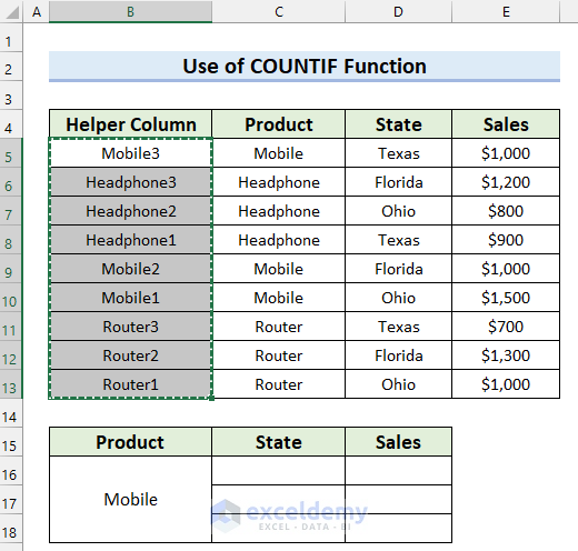
7. Use of COUNTIF Function to VLOOKUP with Multiple Results

In this example, I will show you how you can use the COUNTIF function to use the VLOOKUP function with multiple criteria and multiple results in Excel. For this example, I have taken the following dataset. This dataset contains Product, State, and Sales. This table contains multiple matches for the same product. I will show you how you can get all the results by using the VLOOKUP function.

Let’s see the steps.

Steps:

Firstly, create a Helper Column. In this column, I will give unique names for all the products.

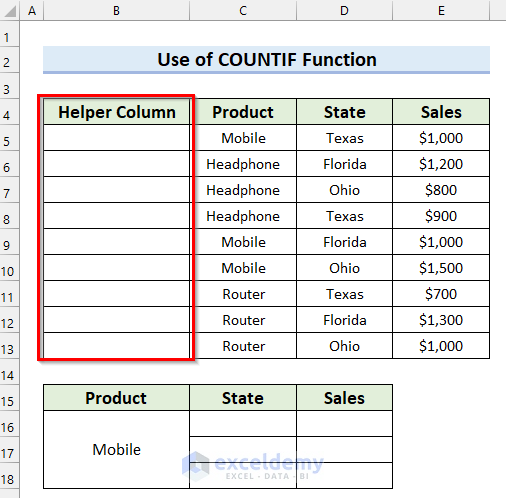
Secondly, select the first cell of the Helper Column. Here, I selected cell B5.
Thirdly, in cell B5 write the following formula.

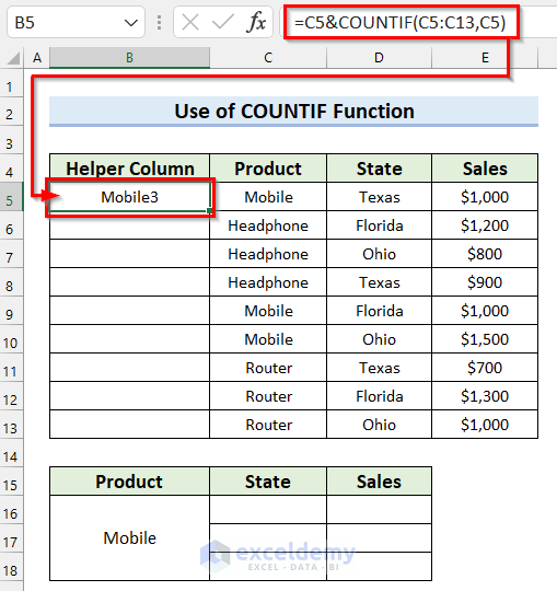
=C5&COUNTIF(C5:C13,C5)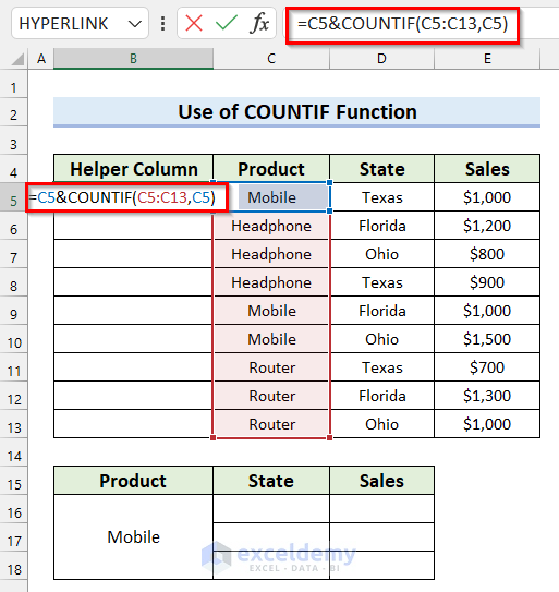

Here, in the COUNTIF function, I selected cell range C5:C13 as the range and cell C5 as the criteria. Now, the function will return the number of cells that match the criteria. Finally, the Ampersand Operator will join the text and formula.

After that, press ENTER to get the result.

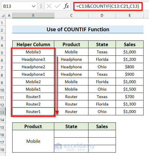
Next, drag the Fill Handle to copy the formula.

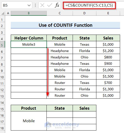
Here, you can see that I have copied the formula to all the other cells and got unique names for every Product.

After that, I will keep only the value to ignore the Circular Reference error.

Firstly, select the cell range. Here, I selected cell range B5:B13.
Secondly, copy the cell range by pressing CTRL+C on your keyboard.

Thirdly, Right-click on the selected range.
After that, select Values from the Paste Options.

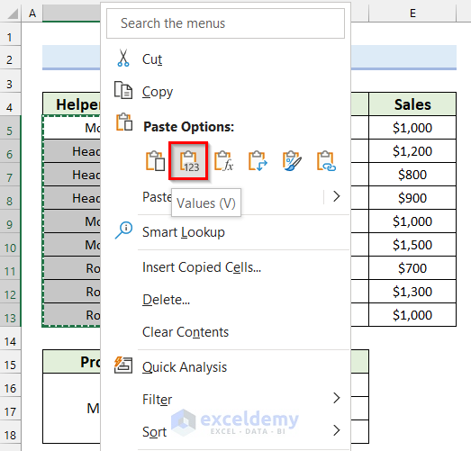
Now, you will see that the cells contain only values, not formulas.

Here, I will use the VLOOKUP function to find multiple results for a specific Product.

Firstly, select the cells from where you want to start the multiple results. Here, I selected cell C16.
Secondly, in cell C16 write the following formula.

=VLOOKUP(B16&ROW(A1:A3),B5:E13,3,FALSE)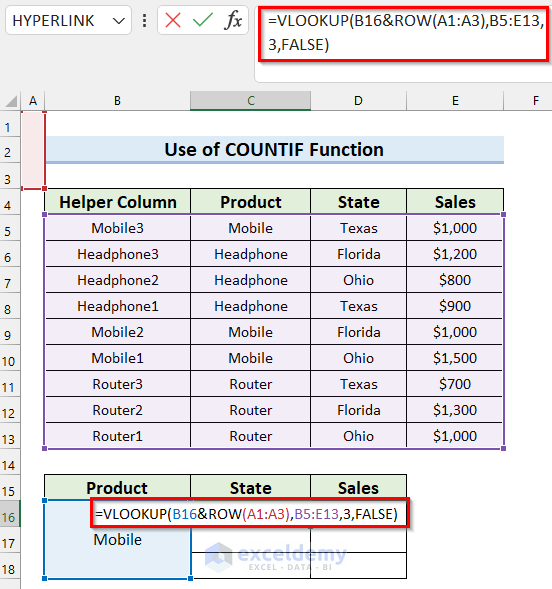

Formula Breakdown

ROW(A1:A3) —-> Here, the ROW function will return the row numbers of the selected cell range.
- Output: {1;2;3}
B16&ROW(A1:A3) —-> turns into
- B16&{1;2;3} —-> Here, the Ampersand Operator will join the text with the formula.
  - Output: {“Mobile1″;”Mobile2″;”Mobile3”}
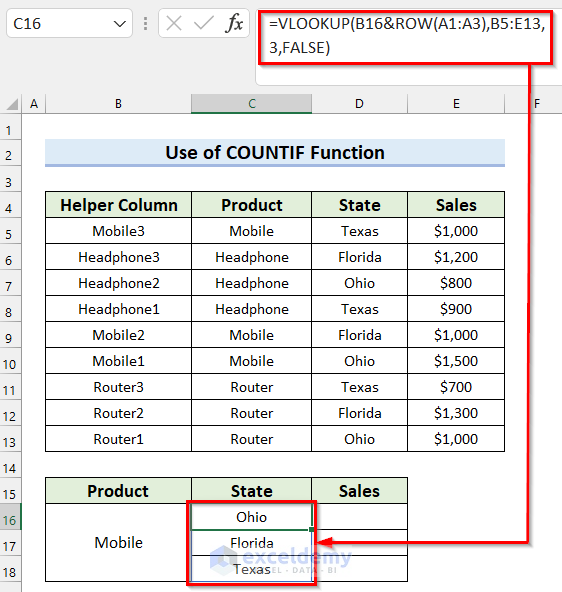
VLOOKUP(B16&ROW(A1:A3),B5:E13,3,FALSE) —-> turns into
- VLOOKUP({“Mobile1″;”Mobile2″;”Mobile3”},B5:E13,3,FALSE) —-> Here, the VLOOKUP function will find match for multiple lookup_values and return multiple results as an array.
  - Output: {“Ohio”;”Florida”;”Texas”}

After that, press ENTER to get the result. If you are using an older version of Microsoft Excel than Excel 2019, then press CTRL+SHIFT+ENTER to get the results.

Now, I will show you how you can find all the Sales for Mobile.

Firstly, select the cell from where you want to start the Sales. Here, I selected cell D16.
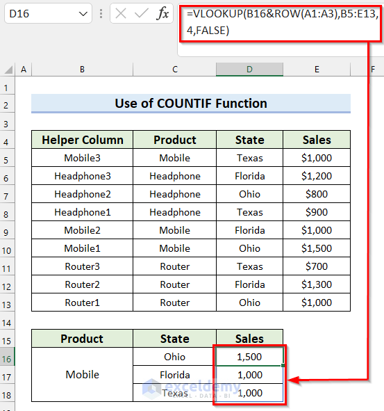
Secondly, in cell D16 write the following formula.

=VLOOKUP(B16&ROW(A1:A3),B5:E13,4,FALSE)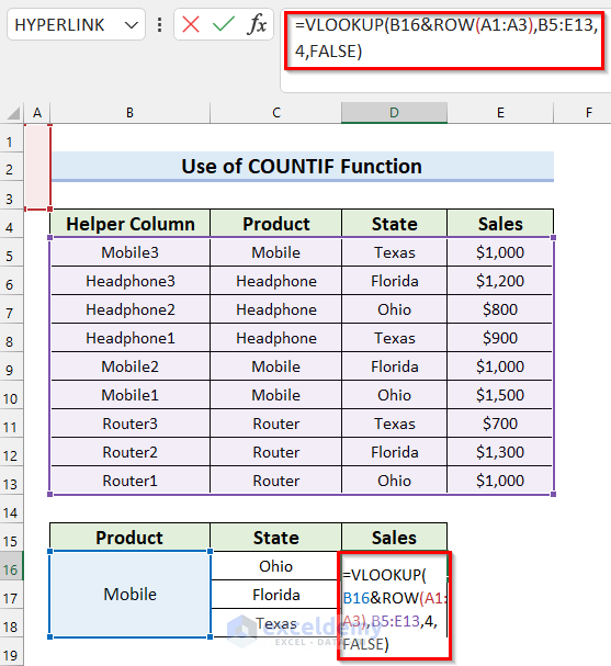

Formula Breakdown

ROW(A1:A3) —-> Here, the ROW function will return the row numbers of the selected cell range.
- Output: {1;2;3}
B16&ROW(A1:A3) —-> turns into
- B16&{1;2;3} —-> Here, the Ampersand Operator will join the text with the formula.
  - Output: {“Mobile1″;”Mobile2″;”Mobile3”}
VLOOKUP(B16&ROW(A1:A3),B5:E13,4,FALSE) —-> turns into
- VLOOKUP({“Mobile1″;”Mobile2″;”Mobile3”},B5:E13,4,FALSE) —-> Here, the VLOOKUP function will find match for multiple lookup_values and return multiple results as an array.
  - Output: {1500;1000;1000}

Finally, press ENTER to get the result. If you are using an older version of Microsoft Excel than Excel 2019, then press CTRL+SHIFT+ENTER to get the results.

8. VLOOKUP with Multiple Criteria and Multiple Results

In this example, I will show you how you can do VLOOKUP with multiple criteria and multiple results without using the VLOOKUP function. Here, I will use the IFERROR, INDEX, SMALL, IF and ROW functions to get the same result as VLOOKUP with multiple criteria and multiple results.

For example, you have a dataset containing the State, the Product, and the Sales Person columns. Now, I will show you how you can find the names of the Sales Person who sell a specific Product in a specific State.

Let’s see the steps.

Steps:

Firstly, select the cell from where you want to start the multiple results. Here, I selected cell H5.
Secondly, in cell H5 write the following formula.

=IFERROR(INDEX($D$5:$D$14, SMALL(IF(1=((--($F$5=$B$5:$B$14)) * (--($G$5=$C$5:$C$14))), ROW($D$5:$D$14)-4,""), ROW()-4)),"")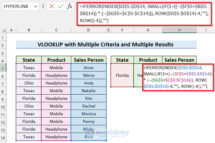

Formula Breakdown

(–($F$5=$B$5:$B$14)) —-> Here, the Double Unary Operator will return the True False values as Zeros and Ones.
- Output: {0;1;0;0;1;0;0;1;1;0}
(–($G$5=$C$5:$C$14)) —-> Now, the Double Unary Operator will return the True False values as Zeros and Ones.
- Output: {0;1;1;0;1;0;0;0;1;1}
((–($F$5=$B$5:$B$14)) * (–($G$5=$C$5:$C$14))) —-> turns into
- ({0;1;0;0;1;0;0;1;1;0} * {0;1;1;0;1;0;0;0;1;1}) —-> Here, these two arrays will be multiplied.
  - Output: {0;1;0;0;1;0;0;0;1;0}
ROW($D$5:$D$14)-4 —-> Here, the ROW function will return the row numbers of the selected cell range and then subtract 4 from the numbers.
- Output: {1;2;3;4;5;6;7;8;9;10}
IF(1=((–($F$5=$B$5:$B$14)) * (–($G$5=$C$5:$C$14))), ROW($D$5:$D$14)-4,””) —-> turns into
- IF(1={0;1;0;0;1;0;0;0;1;0}, {1;2;3;4;5;6;7;8;9;10},””) —-> Next, the IF function will check for the logical_test. If it is True then the function will return numbers from the array otherwise it will return a blank.
  - Output: {“”;2;””;””;5;””;””;””;9;””}
ROW()-4 —-> Now, the ROW function will return the row number of the cell it is in and then subtract 4 from the number.
- Output: {1}
SMALL(IF(1=((–($F$5=$B$5:$B$14)) * (–($G$5=$C$5:$C$14))), ROW($D$5:$D$14)-4,””), ROW()-4) —-> turns into
- SMALL({“”;2;””;””;5;””;””;””;9;””}, {1}) —-> Here, the SMALL function will return a numeric value from the array based on the position in ascending order.
  - Output: {2}
INDEX($D$5:$D$14, SMALL(IF(1=((–($F$5=$B$5:$B$14)) * (–($G$5=$C$5:$C$14))), ROW($D$5:$D$14)-4,””), ROW()-4)) —-> turns into
- INDEX($D$5:$D$14, {2}) —-> Here, the INDEX function will return the value in the given position of the array.
  - Output: “Merry”
IFERROR(INDEX($D$5:$D$14, SMALL(IF(1=((–($F$5=$B$5:$B$14)) * (–($G$5=$C$5:$C$14))), ROW($D$5:$D$14)-4,””), ROW()-4)),””) —-> turns into
- IFERROR(“Merry”,””) —-> Here, the IFERROR function will return blank if any error is found.
  - Output: “Merry”

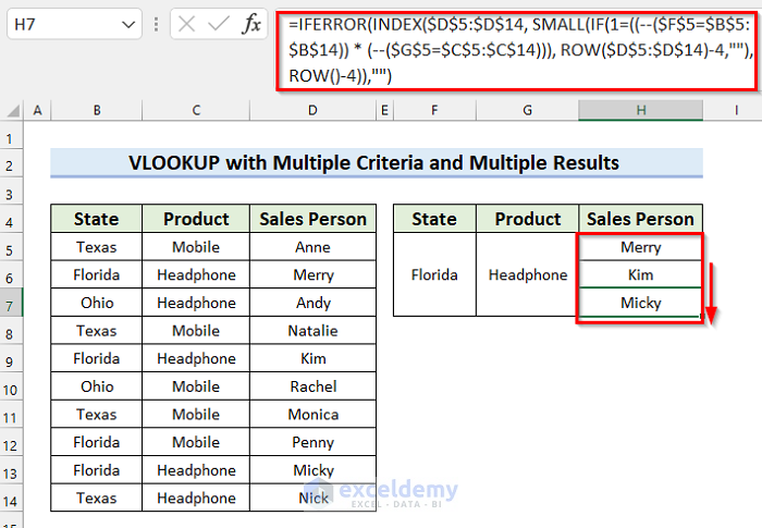
Finally, press ENTER to get the result.

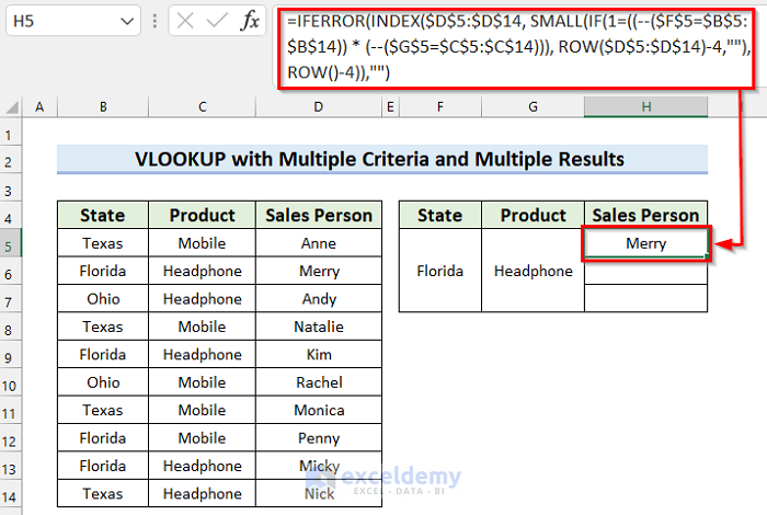
After that, drag the Fill Handle to other results for the same criteria.

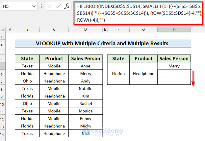
Finally, You can see that I have got all the names of the Sales Person who sells Headphones in Florida.

How to Combine VLOOKUP with Other Functions in Excel

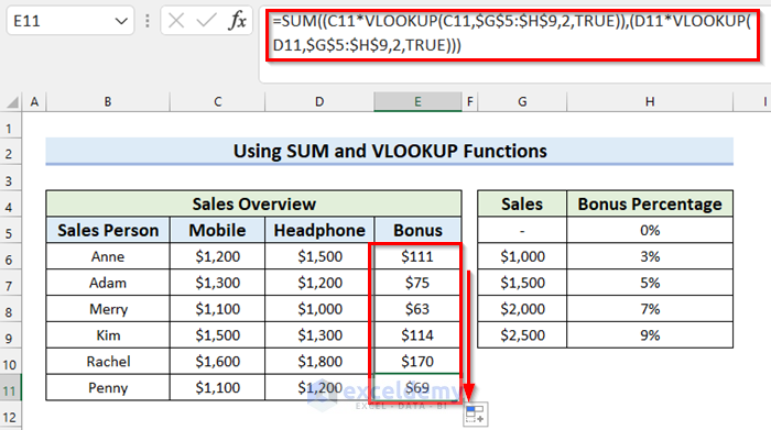
In this section, I will show you how you can combine the VLOOKUP function with other functions in Excel to get your desired result. Here, I will show 2 different examples. The first one is for combining the VLOOKUP function with the SUM function and the other one is for combining the SUMIF function with VLOOKUP.

1. Using SUM and VLOOKUP Functions

In this example, I will use the SUM function and the VLOOKUP function together. For this example, I have taken the following dataset. The dataset contains Sales Person and Sales for the Products they sold. Here, I will use the VLOOKUP function to find the Bonus Percentage for that specific Sales amount. And then use the SUM function to calculate the Bonus.

Let’s see the steps.

Steps:

Firstly, select the cell where you want to calculate the Bonus. Here, I selected cell E6.
Secondly, in cell E6 write the following formula.

=SUM((C6*VLOOKUP(C6,$G$5:$H$9,2,TRUE)),(D6*VLOOKUP(D6,$G$5:$H$9,2,TRUE)))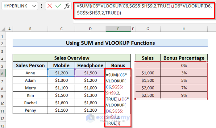

Formula Breakdown

VLOOKUP(C6,$G$5:$H$9,2,TRUE) —-> Here, the VLOOKUP function will look for a match from the table_array and then return the result from column 2.
- Output: 0.03
VLOOKUP(D6,$G$5:$H$9,2,TRUE) —-> Now, the VLOOKUP function will look for a match from the table_array and then return the result from column 2.
- Output: 0.05
(C6*VLOOKUP(C6,$G$5:$H$9,2,TRUE)) —-> turns into
- (C6*0.03) —-> Here, the value in cell C6 will be multiplied by 0.03.
  - Output: 36
(D6*VLOOKUP(D6,$G$5:$H$9,2,TRUE)) —-> turns into
- (D6*0.05) —-> Here, the value in cell D6 will be multiplied by 0.05.
  - Output: 75
SUM((C6*VLOOKUP(C6,$G$5:$H$9,2,TRUE)),(D6*VLOOKUP(D6,$G$5:$H$9,2,TRUE))) —-> turns into
- SUM(36,75) —-> Now, the SUM function will return the summation of these values.
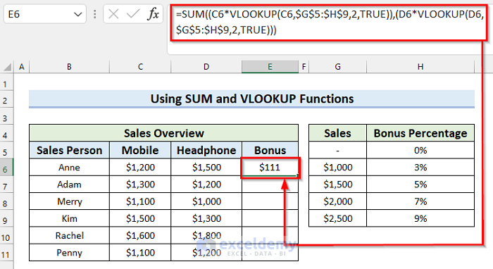
  - Output: 111

Finally, press ENTER to get the result.

After that, drag the Fill Handle to copy the formula to the other cells.

Here, you can see that I have copied the formula to the other cells and calculated the Bonus for every Sales Person.

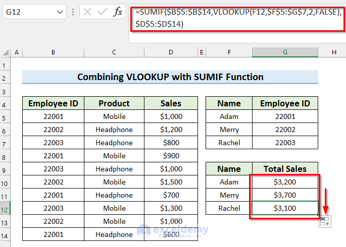
2. Combining VLOOKUP Function with SUMIF Function

In this example, I will combine the VLOOKUP function with the SUMIF function. Suppose you want to calculate the Total Sales for every employee. You can calculate this type of calculation by using the SUMIF function. But, here, you want the Total Sales against their Name but your dataset contains the Employee ID. So, I will use the VLOOKUP function to find the Employee ID of the salesperson and then use the SUMIF function.

Let’s see the steps.

Steps:

Firstly, select the cell where you want the Total Sales. Here, I selected cell G10.
Secondly, in cell G10 write the following formula.

=SUMIF($B$5:$B$14,VLOOKUP(F10,$F$5:$G$7,2,FALSE),$D$5:$D$14)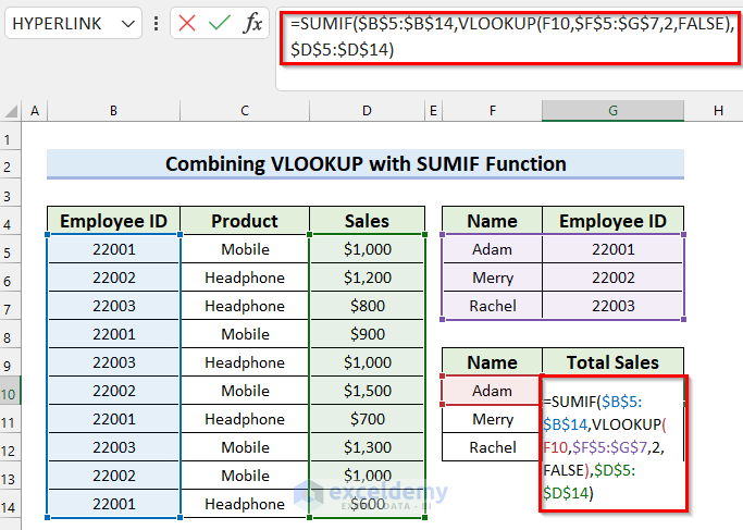

Formula Breakdown

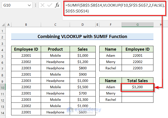
VLOOKUP(F10,$F$5:$G$7,2,FALSE) —-> Here, the VLOOKUP function will look for a match for the look_up value and return the Employee ID.
- Output: 22001
SUMIF($B$5:$B$14,VLOOKUP(F10,$F$5:$G$7,2,FALSE),$D$5:$D$14) —-> turns into
- SUMIF($B$5:$B$14,22001,$D$5:$D$14) —-> Now, the SUMIF function will sum the values from sum_range that match the criteria.
  - Output: 3200

Thirdly, press ENTER to get the Total Sales.

After that, drag the Fill Handle to copy the formula to the other cells.

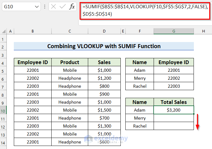
Finally, you can see that I have copied the formula for all the cells and got the Total Sales for every employee.

Things to Remember

In cases of an array formula, you will have to press CTRL+SHIFT+ENTER if you are using an older version of Microsoft Excel than Excel 2019.

Practice Section

Here, I have provided a practice sheet for you to practice using VLOOKUP with multiple criteria and multiple results.

Download Practice Workbook

Using VLOOKUP Function with Multiple Criteria and Results.xlsx

Conclusion

In this article, I tried to cover how to use VLOOKUP with multiple criteria and multiple results. Here, I explained 8 different examples. I hope this article was clear to you. Lastly, if you have any questions, feel free to let me know in the comment section below.

<< Go Back to VLOOKUP with Multiple Criteria | Excel VLOOKUP Function | Excel Functions | Learn Excel

Get FREE Advanced Excel Exercises with Solutions!

VLOOKUP with Multiple Criteria and Multiple Results (8 Examples)

How to Use VLOOKUP with Multiple Criteria and Multiple Results: 8 Suitable Examples

1. Using Ampersand Operator to VLOOKUP with Multiple Criteria

2. Applying CONCATENATE Function to VLOOKUP with Multiple Criteria and Return Multiple Results

3. Employing CHOOSE Function to VLOOKUP with Multiple Criteria

4. Using MAX and VLOOKUP Functions with Multiple Criteria to Return Multiple Results

5. Applying MATCH and VLOOKUP Functions for Multiple Criteria

6. Using IF & VLOOKUP Functions with Multiple Criteria and Multiple Results

7. Use of COUNTIF Function to VLOOKUP with Multiple Results

8. VLOOKUP with Multiple Criteria and Multiple Results

How to Combine VLOOKUP with Other Functions in Excel

1. Using SUM and VLOOKUP Functions

2. Combining VLOOKUP Function with SUMIF Function

Things to Remember

Practice Section

Conclusion

Related Articles

Leave a reply Cancel reply