Methods 1 – Insert Ampersand Inside Excel VLOOKUP to Join with Multiple Criteria in Column and Row
STEPS:
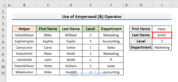
- Insert a Helper column on the leftmost side of the table or range like the picture below.
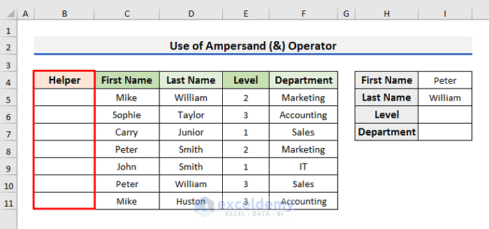
Note: The range B4:E11 was the main dataset. After adding a Helper column, the range B4:F11 becomes the new dataset.
- Select Cell B5 and type the formula below:
=C5&D5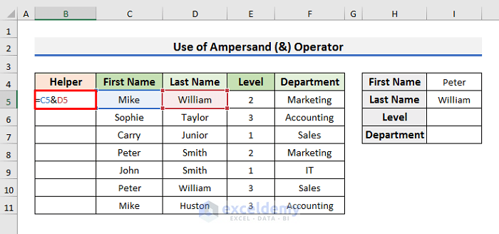
We have used the Ampersand (&) operator to concatenate the texts of Cell C5 and Cell D5.
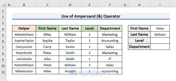
- Press Enter and drag the Fill Handle down to copy the formula till Cell B13.
- Select Cell I6 and type the formula below:
=VLOOKUP($I$4&$I$5,$B$5:$F$11,4,FALSE)- Hit Enter to see the result.
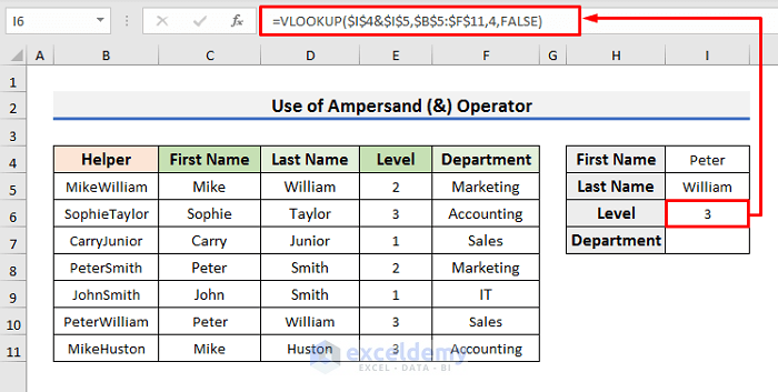
This VLOOKUP formula looks for the value PeterWilliam in the range B5:F11 and extracts the Level value.
How Does the Formula Work?
- In this formula, the first argument ($I$4&$I$5) denotes PeterWilliam which is the lookup value. We have used absolute cell reference to lock the cells.
- The second argument ($B$5:$F$11) is the lookup array where the formula will search for the lookup value.
- We want to extract the desired Level value that is situated in the fourth column of the range B4:F11. We have typed 4 in the third argument.
- As we needed the exact match, we typed FALSE in the fourth argument.
- Get the value of the Department, type the formula below in Cell I7:
=VLOOKUP($I$4&$I$5,$B$5:$F$11,5,FALSE)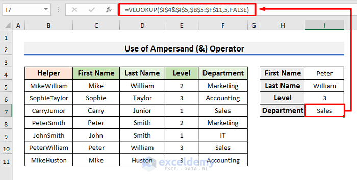
We have changed the Column Index Number to 5 as Department is the fifth column of the range B4:F11.
- If you change the Last Name, the Level and Department will automatically update.
Method 2 – Excel VLOOKUP with CHOOSE Function to Add Multiple Criteria in Column and Row
STEPS:
- Select Cell H6 and type the formula below:
=VLOOKUP($H$4&$H$5,CHOOSE({1,2},$B$5:$B$11&$C$5:$C$11,$D$5:$D$11),2,FALSE)- Press Enter to see the Level of Peter William.
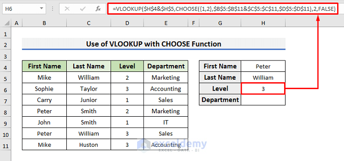
We have used the CHOOSE function in the second argument of the VLOOKUP function. The CHOOSE function forms a table with Columns B, C, and D. In that table, Columns B and C are merged and Column D is the second column. The VLOOKUP formula looks for the value of Cell H4 and Cell H5 inside the newly formed table and extracts the row from the second column of that table. That is how we get the Level value of Peter William.
- Type the formula below in Cell H7 to get the Department name:
=VLOOKUP($H$4&$H$5,CHOOSE({1,2},$B$5:$B$11&$C$5:$C$11,$E$5:$E$11),2,FALSE)- Press Enter to see the Department of Peter William.
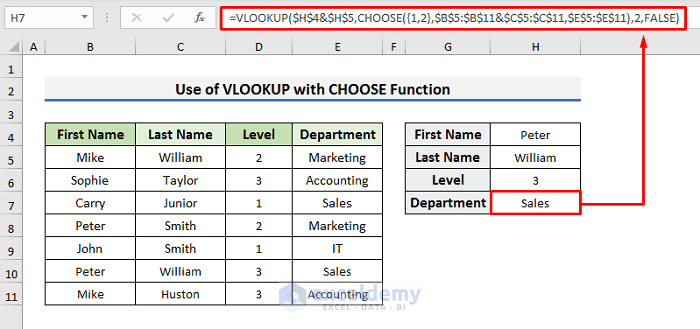
We have used $E$5:$E$11 in place of $D$5:$D$11. So, the CHOOSE function forms a table with Columns B, C, and E this time.
Method 3 – Join Multiple Criteria in Column and Row by Merging VLOOKUP with IF Function
STEPS:
- Select Cell H6 and type the formula below:
=VLOOKUP(H4,IF(C5:C11=H5,B5:E11,""),3,FALSE)- Press Enter to see the Level value.
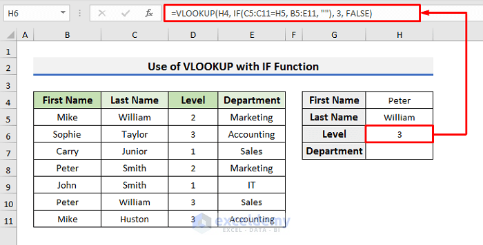
In this formula, the VLOOKUP function looks for the value of Cell H4 if Column C is equal to the value of Cell H5. Extract the row from Column D of the range B5:E11. You can also use the absolute cell reference to lock the cells.
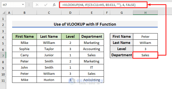
- Select Cell H7 and type the formula below:
=VLOOKUP(H4,IF(C5:C11=H5,B5:E11,""),4,FALSE)- Press Enter to see the Department name in Cell H7.
Method 4 – Apply Excel VLOOKUP with MATCH Function for Multiple Criteria in Column and Row
STEPS:
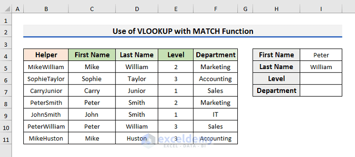
- Add a Helper column in Column B.
- Select Cell B5 and type the formula below:
=C5&D5- Hit Enter and drag the Fill Handle down to copy the formula to Cell B11.
- You will see results like the picture below.
- Select Cell I6 and type the formula below:
=VLOOKUP($I$4&$I$5,B5:F11,MATCH(E4,B4:F4,0),FALSE)- Press Enter to get the Level value.
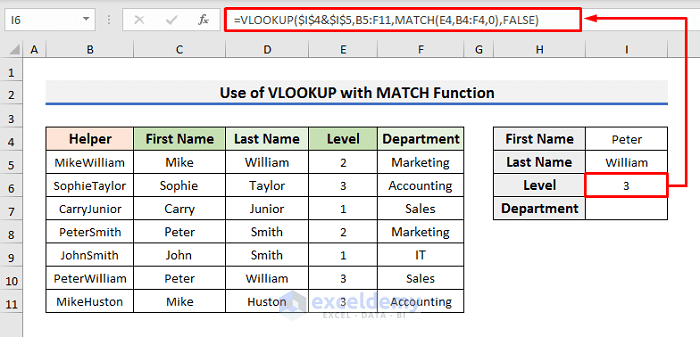
The MATCH function returns the column index number of Cell E4, which is 4. So, the VLOOKUP formula becomes:
=VLOOKUP($I$4&$I$5,B5:F11,4,FALSE)
which is the same as the formula of Example 1.
- Get the Department name, type the formula below in Cell I7:
=VLOOKUP($I$4&$I$5,B5:F11,MATCH(F4,B4:F4,0),FALSE)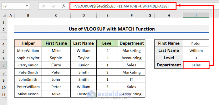
The difference between this formula and the previous one is the part of the MATCH function. We have used the MATCH function to look for the column index number of Cell F4 in the range B4:F4. This returns 5. This formula is also similar to the last formula of Example 1.
Method 5 – Use Excel VLOOKUP Function with Multiple Criteria in Single Column
STEPS:
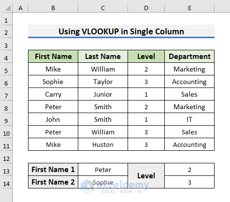
- Select Cell E13 and type the formula below:
=VLOOKUP(C13:C14,B5:E11,3,FALSE)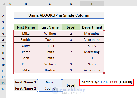
- Press Ctrl + Shift + Enter to see the Level number of Peter and Sophie.
Note: This formula has a drawback. The VLOOKUP function always extracts the first matched data, which is why we are getting the Level value of Peter Smith, not of Peter William.
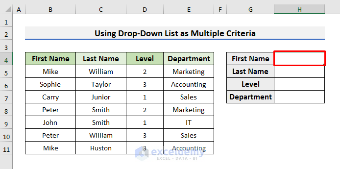
Method 6 – Insert Drop-Down Lists as Multiple Criteria in VLOOKUP
STEPS:
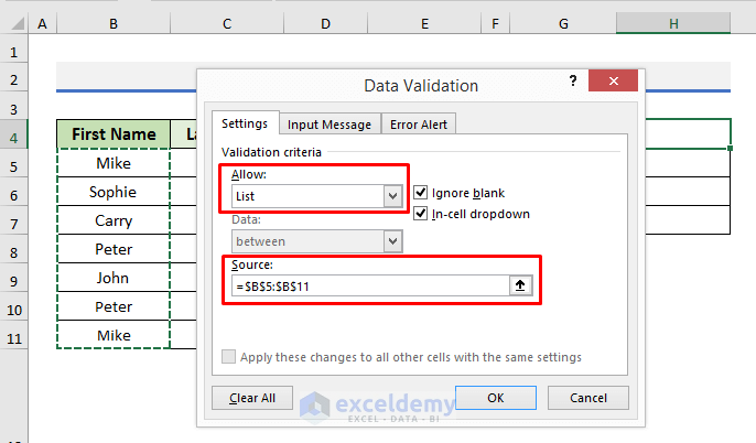
- Select Cell H4.
- Go to the Data tab and click on the Data Validation option. A dialog box will appear.

- Select List in the Allow field.
- Enable editing in the Source box and select the range B5:B11.
- Click OK to proceed.
- You will see a drop-down list in Cell H4.
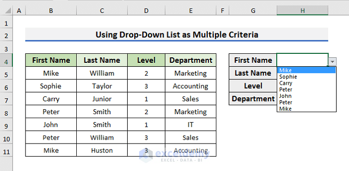
- Repeat the same steps to get a drop-down list in Cell H5.
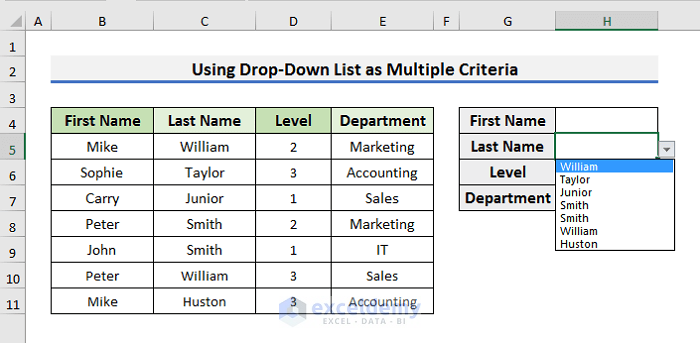
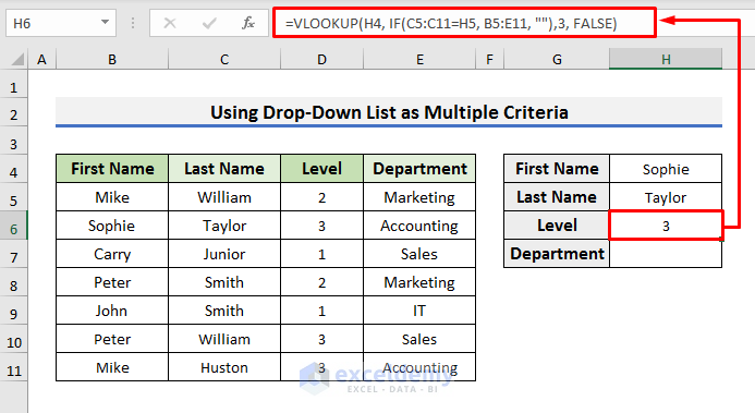
- Select the First and Last Names using the drop-down lists.
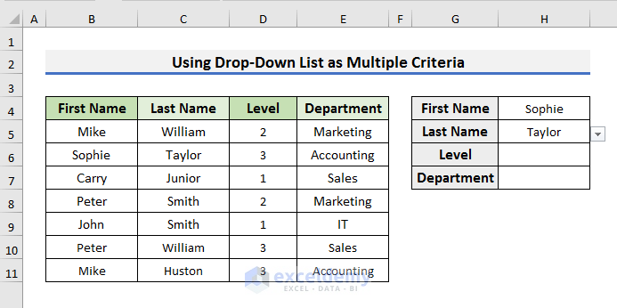
- Select Cell H6 and type the formula below to get the Level value:
=VLOOKUP(H4,IF(C5:C11=H5,B5:E11,""),3,FALSE)- Press Enter to see the result.
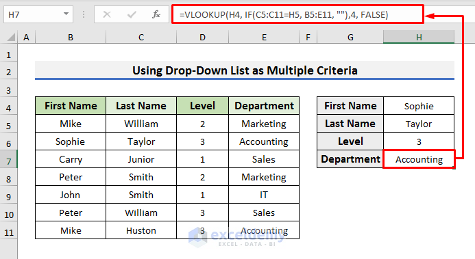
- Type the formula below in Cell H7 to find the Department name:
=VLOOKUP(H4,IF(C5:C11=H5,B5:E11,""),4,FALSE)- Hit Enter for the result.
Note: We have used this VLOOKUP with the IF function formula in Example 3. You can find the explanation there.
Download Practice Workbook
You can download the practice workbook from here.
Related Articles
<< Go Back to VLOOKUP with Multiple Criteria | Excel VLOOKUP Function | Excel Functions | Learn Excel
Get FREE Advanced Excel Exercises with Solutions!
