How to Use VLOOKUP with Multiple Criteria Including a Date Range: 2 Examples

The following dataset will be used. The dataset contains prices of three different products during 3 quarters of the year 2021.

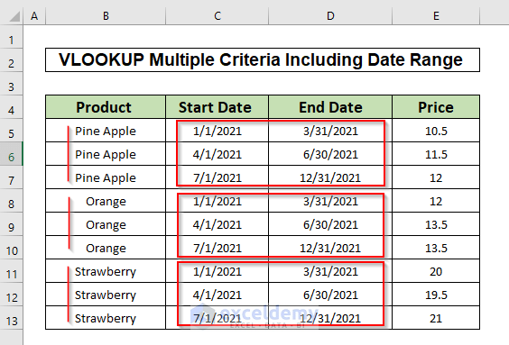
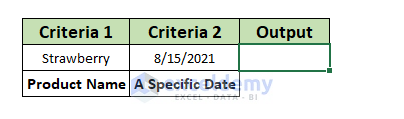
From this dataset, we want to know the price of a product at a specific date.

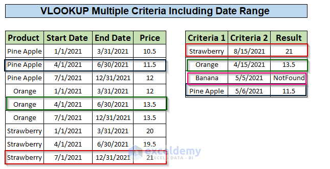
Example 1 – VLOOKUP Multiple Criteria Including Date Range Using the INDEX and MATCH Functions

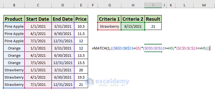
To find the price of Strawberry on 8/15/2021, input the following formula in cell I5.

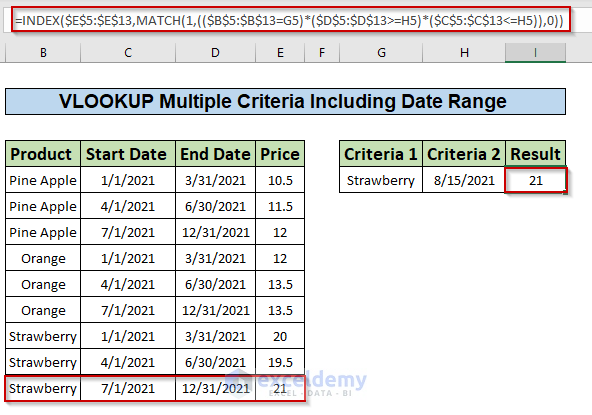
The result is 21 as shown in the screenshot above.

Formula Breakdown:

The INDEX function is used to findthe value of a specific location in a dataset. In this example, we used the MATCH function with the INDEX function. The MATCH function provides the location of the cell (row number) that fulfills both of the criteria.
The INDEX function takes the following arguments:
(array, row_num, [col_num])
The first argument of the INDEX function is $E$5:$E$13 which represents the price column from where we need to find the desired value.

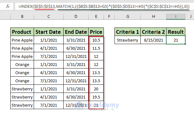
To provide the row number argument of the INDEX function, we use the MATCH function. The MATCH function checks the conditions specified and then outputs the row number of the cell data that fulfills both conditions.

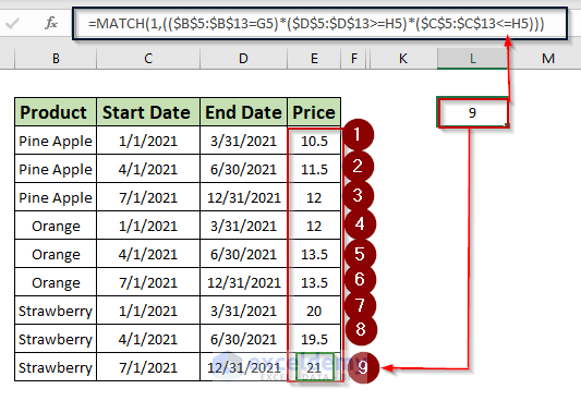
The MATCH function checks three conditions here-
($B$5:$B$13=G5) checks the value Strawberry (G5) in column B.
($D$5:$D$13>=H5)*($C$5:$C$13<=H5) checks whether the date 8/15/2021 lies in between the Start Date and End Date dates for the rows that already met the first condition.

The following screenshot shows some more outputs to understand the example better.

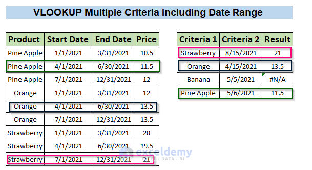
We also tested the formula with the product name “Banana”. This product doesn’t belong to the dataset which is why the output is an #N/A error.

Example 2 – VLOOKUP Multiple Criteria Including Date Range Using the XLOOKUP Function 

Lets find the value of Strawberry’s price on a specific date using the XLOOKUP function. Enter the following formula in cell I5.

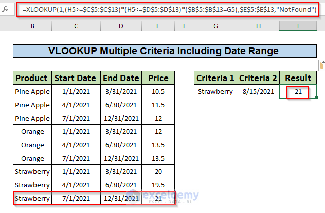
As you can see in the image above, the price was 21,

Formula Breakdown:
The XLOOKUP function is used to lookup for values in a range or array.  It takes several arguments-
(lookup, lookup_array, return_array, [not found])
In this formula, the lookup_array argument represents an array that fulfills three conditions.
(H5>=$C$5:$C$13)*(H5<=$D$5:$D$13) checks whether the date 8/15/2021 lies in between the date range.
($B$5:$B$13=G5) checks the value Strawberry (G5)) in column B and returns the array that already fulfilled the first two conditions.
We also have a string “NotFound”, in case the lookup array doesn’t meet the conditions and returns an empty array.
The following screenshot shows some more outputs to understand the example better.

We also added a product named “Banana” and the formula returned NotFound as our dataset doesn’t contain the product.

Read More:  VLOOKUP with Multiple Criteria and Multiple Results 

Notes

• The XLOOKUP function is a well-suited and more flexible alternative to the VLOOKUP and HLOOKUP. It provides match_mode and search_mode, two different arguments with multiple options that make a lookup for values easy and flexible with different conditions.

Download Practice Workbook

Download this practice workbook to exercise while you are reading this article.

Related Articles

• Excel VLOOKUP with Multiple Criteria in Horizontal & Vertical Way
• Excel VLOOKUP with Multiple Criteria in Column and Row
• Vlookup with Multiple Criteria without a Helper Column in Excel 
• How to Apply VLOOKUP with Multiple Criteria Using the CHOOSE Function
• How to Use VLOOKUP with Multiple Criteria in Different Sheets

<< Go Back to VLOOKUP with Multiple Criteria | Excel VLOOKUP Function | Excel Functions | Learn Excel