Method 1 – Use a Helper Column to Left to Match Multiple Criteria with VLOOKUP
Steps:
- Create a helper column on the left side of your dataset.
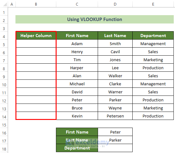
- Click on cell B5.
- Insert the following formula with AND function and hit Enter.
=AND(C5=$D$16,D5=$D$17)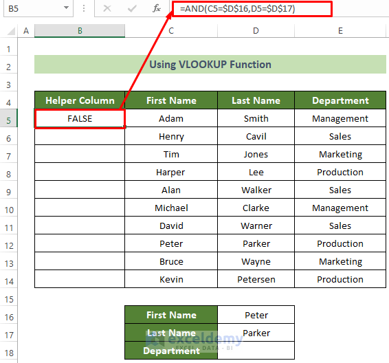
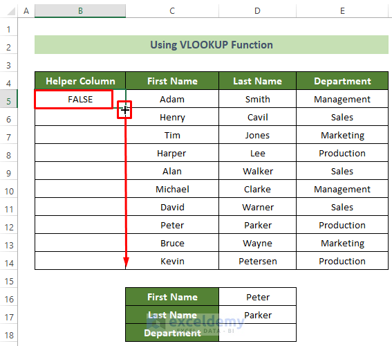
- Place your cursor in the bottom right position of cell B5.
- A black fill handle will appear.
- Drag the fill handle below to copy the same formula for all the cells below.
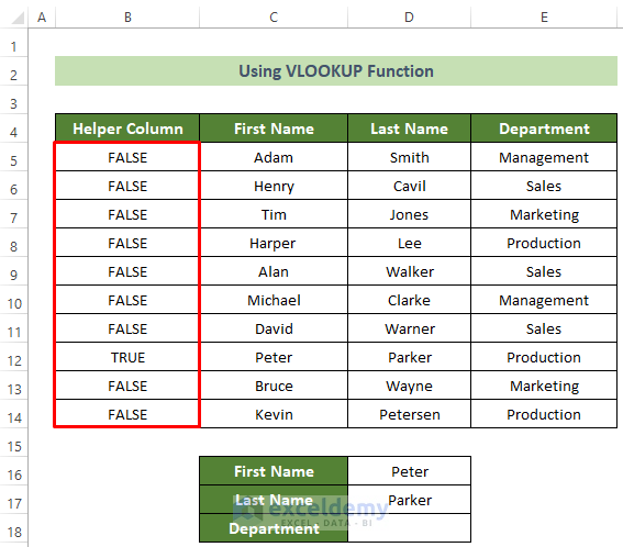
- You will get all the helper column data.
- Click on cell D18 and insert the following formula.
=VLOOKUP(TRUE,B5:E14,4,FALSE)- Press Enter.
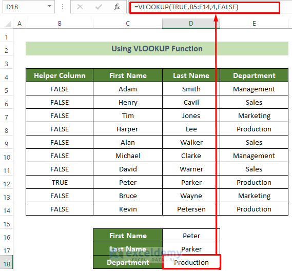
You will be able to look up your desired data in the dataset with multiple criteria horizontally and vertically.
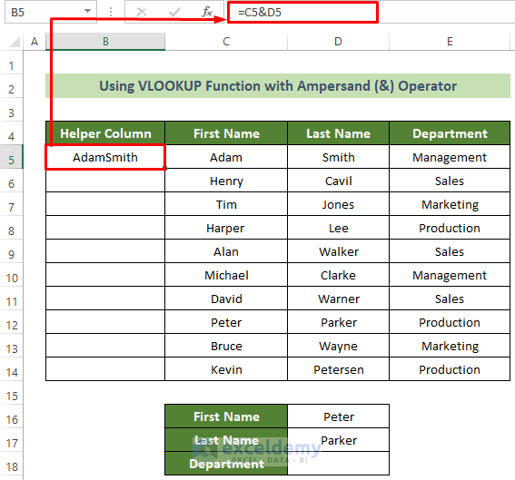
Method 2 – Apply VLOOKUP Function with Multiple Criteria Using Ampersand (&) Operator with Helper Column
Steps:
- Click on cell B5 and insert the following formula in your helper column cell.
=C5&D5- Press Enter.
- Place your cursor in the bottom right position of cell B5 and drag the black fill handle downward to copy the same formula for all the cells below.
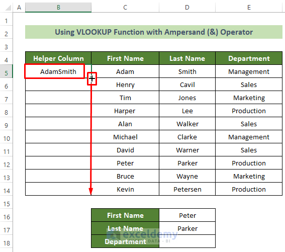
- You will get all the helper column data that fits your needs.
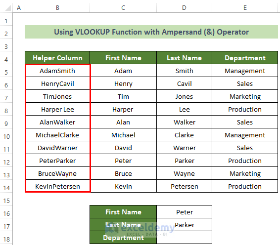
- Click on cell D18 and insert the formula below.
=VLOOKUP(D16&D17,B5:E14,4,FALSE)- Press the Enter button.
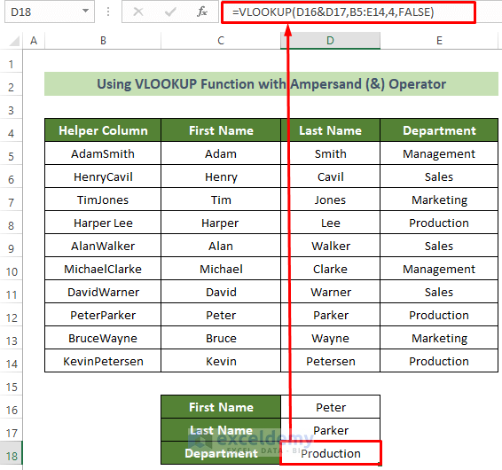
You will get your desired person’s department looked up.
Method 3 – Use Helper Row and Combine TRANSPOSE Function with VLOOKUP for Horizontal Lookup
Steps:
- At the Helper Row, click on cell C4.
- Insert the formula below and press Enter.
=C5&C6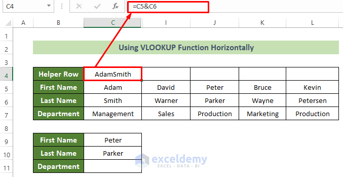
- Place your cursor in the bottom right position of cell C4.
- Drag the fill handle rightward upon its arrival.
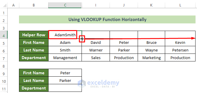
- You will get all the data of the helper row.
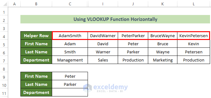
- Click on cell C11 and insert the following formula.
=VLOOKUP(C9&C10,TRANSPOSE(C4:L7),4,FALSE)- Hit the Enter button.
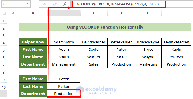
You will get the department for Peter Parker.
How to VLOOKUP for Horizontal and Vertical Lookup with Multiple Criteria in Excel: 2 Alternative Formulas
Method 1 – INDEX-MATCH Formula for Vertical and Horizontal Lookup with Multiple Criteria
Steps:
- Click on cell C18 and insert the following formula.
=INDEX(D5:D14,MATCH(1,(B5:B14=C16)*(C5:C14=C17),0))Formula Breakdown:
- MATCH(1,(B5:B14=C16)*(C5:C14=C17)
This function will return the row index number where the C16 cell’s value is in the B5:B14 range and the C17 cell’s value is in the C5:C14 range.
Result: 8
- INDEX(D5:D14,MATCH(1,(B5:B14=C16)*(C5:C14=C17),0))
This function returns the value from the D5:D14 cells for the previous row index result.
Result: Production
- Hit Enter.
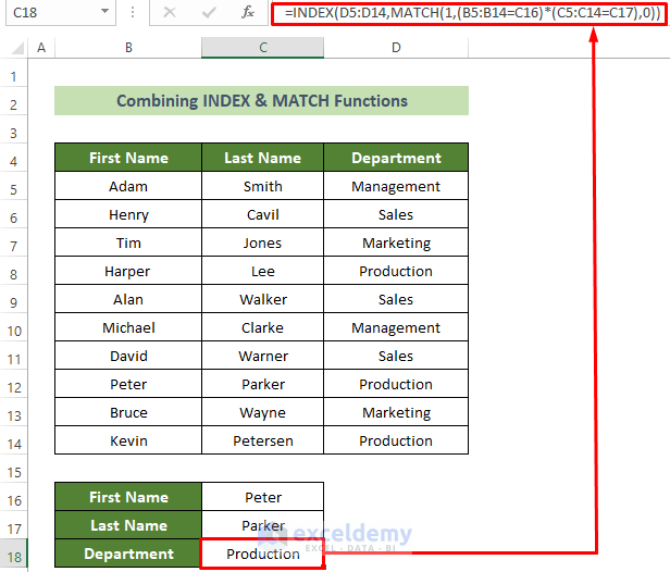
You can get the desired result for your desired salesperson.
Lookup Horizontally:
Steps:
- Click on cell C10.
- Insert the following formula and press the Enter button.
=INDEX(C6:L6,MATCH(1,(C4:L4=C8)*(C5:L5=C9),0))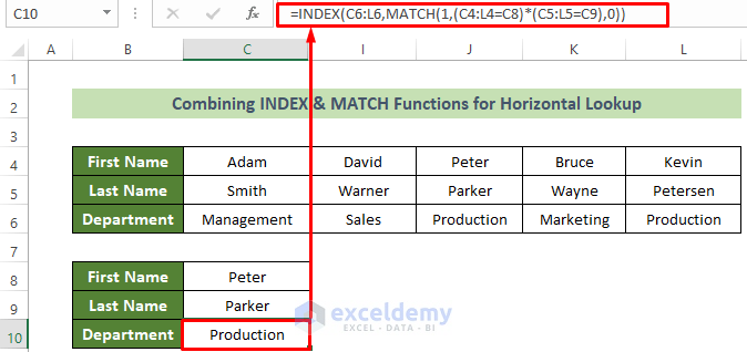
You can get the desired person’s department by horizontal lookup.
Method 2 – Using XLOOKUP Function to Lookup Vertically and Horizontally with Multiple Criteria
Steps:
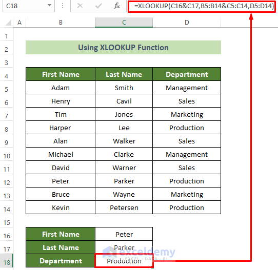
- Click on cell C18 and insert the following formula.
=XLOOKUP(C16&C17,B5:B14&C5:C14,D5:D14)- Hit Enter.
Steps:
- Click cell C10.
- Insert the following formula.
=XLOOKUP(C8&C9,C4:L4&C5:L5,C6:L6)- Hit Enter.

You can get your desired result.
Download Practice Workbook
You can download our practice workbook from here for free!
Related Articles
- How to Apply VLOOKUP with Multiple Criteria Using the CHOOSE Function
- How to Use VLOOKUP with Multiple Criteria in Different Sheets
<< Go Back to VLOOKUP with Multiple Criteria | Excel VLOOKUP Function | Excel Functions | Learn Excel
Get FREE Advanced Excel Exercises with Solutions!

