Vlookup with Multiple Criteria without a Helper Column in Excel: 5 Methods

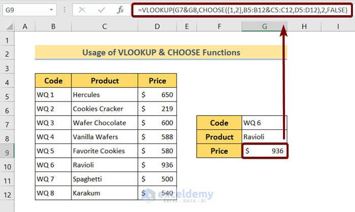
Method 1 – Combine the VLOOKUP and CHOOSE Functions to Vlookup with Multiple Criteria in Excel

❶ Select cell G9 first.

❷ Then insert the following formula:

• G7&G8 are cells where the criteria are.
• CHOOSE({1,2} creates a virtual function of two columns. The first column has the merged content of the cells G7&G8. The second column has the values from cell D5:D12.
• B5:B12 is the range to look for the content of cell G7.
• C5:C12 is the range to look for the content of cell G8.
• D5:D12 is the range to extract the output.
• 2 is the column index number of the virtual table to extract the output.
• FALSE denotes the exact match.

❸ Hit the ENTER button to get the vlookup result.

Using older versions of Microsoft Excel except Office 365, press CTRL + SHIFT + ENTER to insert the formula.

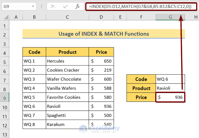
Method 2 – Combine the INDEX and MATCH Functions to Vlookup without a Helper Column in Excel

❶ Click on cell G9 to insert the following formula:

Here,

• D5:D12 is the range of cells to extract the output of vlookup.
• G7&G8 is the cell where the multiple criteria are stated.
• B5:B12&C5:C12 is the range of cells to look for the criteria.
• MATCH(G7&G8,B5:B12&C5:C12,0) searches for matches in between B5:B12&C5:C12 with G7&G8
• INDEX(D5:D12,MATCH(G7&G8,B5:B12&C5:C12,0)) searches for matches in between B5:B12&C5:C12 with G7&G8 respectively and returns the output from D5:D12.

❷ Press the ENTER button to get the vlookup value.

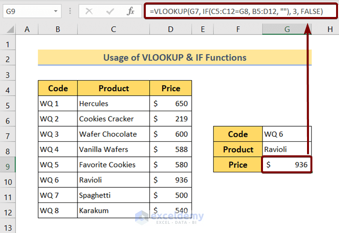
Method 3 – Combine the VLOOKUP and IF Functions to Vlookup with Multiple Criteria

❶ Select a cell first.

❷ Then insert the following formula:

In this formula,

• G7 contains the first criterion.
• C5:C12=G8 looks for the value stored in cell G8 within the range C5:C12.
• B5:D12 is the table array.
• IF(C5:C12=G8, B5:D12, “”) checks if there’s a match between G8 and C5:C12. If there’s a match it returns the value from B5:D12. Otherwise, it returns nothing.
• 3 is the column index number of the table array to get the output.
• FALSE refers exact match.
• VLOOKUP(G7, IF(C5:C12=G8, B5:D12, “”), 3, FALSE) checks if there’s a match between G8 and C5:C12. If there’s a match it returns the value from the 3rd column of B5:D12. Otherwise, it returns a null value.

❸ Finally, hit the ENTER button to get the output vlookup value.

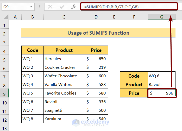
Method 4 – Use the SUMIFS Function to Vlookup with Multiple Criteria in Excel

❶ Insert the following formula in cell G9.

Here,

• D:D refers to the cell range to extract the output value.
• B:B refers to a source data column.
• G7 contains the first criteria.
• C:C refers to another source data column.
• G8 contains the second criteria.

❷ Hit the ENTER button.

Get the vlookup data in cell G9.

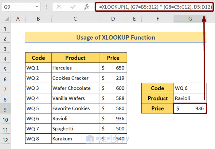
Method 5 – Use the XLOOKUP Function to Vlookup with Multiple Criteria without a Helper Column

❶ Select a cell.

❷ Insert the following formula in that cell:

In this formula,

• G7=B5:B12 looks for the content of G7 in the range B5:B12.
• G8=C5:C12 looks for the content of G8 in the range C5:C12.
• D5:D12 is the cell range to get the output value.
• 1 is the lookup value.

❸ Hit the ENTER button to get the vlookup data in cell G9.

Download Practice Workbook

You can download the Excel file from the following link and practice along with it.

Related Articles

• How to Apply VLOOKUP with Multiple Criteria Using the CHOOSE Function
• How to Use VLOOKUP with Multiple Criteria in Different Sheets

<< Go Back to VLOOKUP with Multiple Criteria | Excel VLOOKUP Function | Excel Functions | Learn Excel