Whilst working in Microsoft Excel, we’ve all faced a scenario where we need to look up a value from a dataset based on a few criteria. Now, even with a small dataset, this is time-consuming and prone to errors, let alone a large dataset. Granted this, the following tutorial aims to demonstrate how you can use VLOOKUP with multiple criteria in different columns.
How to Use VLOOKUP with Multiple Criteria in Different Columns: 5 Ways
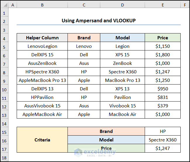
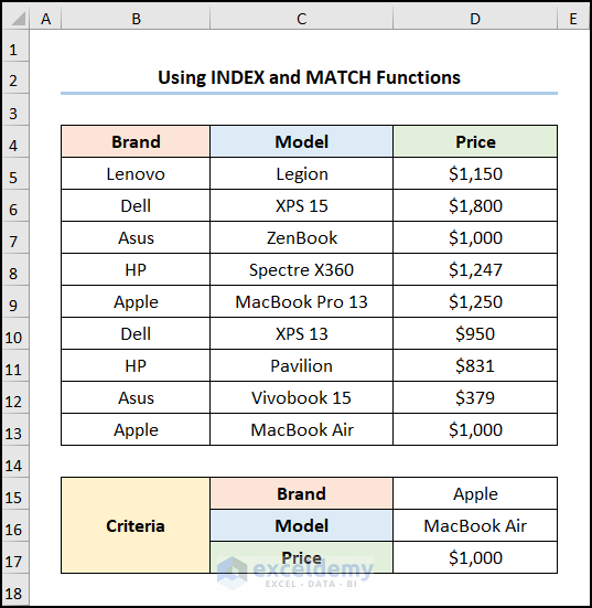
Now, let us consider the List of laptop Prices dataset shown in the B4:D13 cells. Here, we have the Brand, Model, and Prices of each laptop respectively. Now, we want to enter the Brand and Model names to automatically look up the Prices for the corresponding laptop. Therefore, without further delay, let us look at each method one by one.
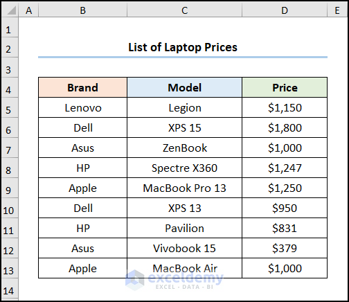
Here, we have used Microsoft Excel 365 version, you may use any other version according to your convenience.
Method-1: Using Ampersand and VLOOKUP
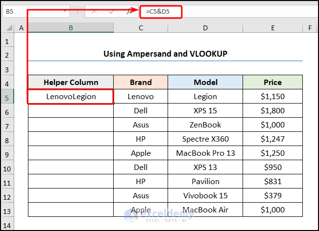
Let us begin with a simple way to retrieve a value according to given conditions. Here, we’ll insert a Helper Column on the left since the VLOOKUP function looks for a value starting from the first column.
📌 Steps:
- At the very beginning, insert a Helper Column >> enter the given formula in the B5 cell to combine the string of texts.
=C5&D5
Here, the C5 and D5 cells refer to the Brand and Model of the laptops respectively.
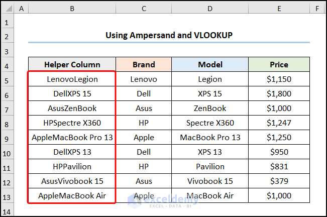
- Then, use the Fill Handle Tool to copy the formula into the cells below.
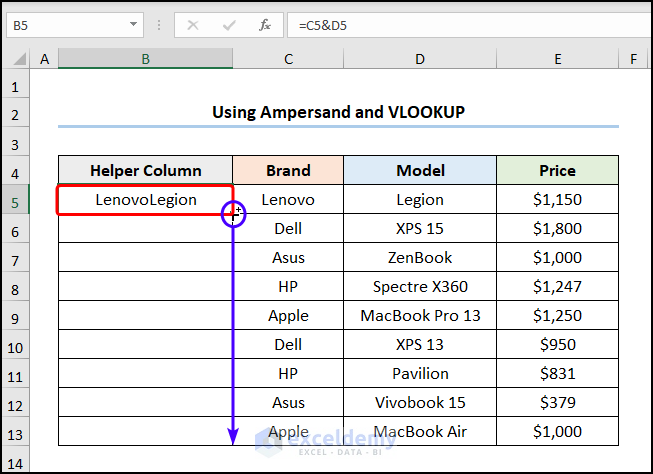
After completing the above steps, the Helper Column should look like the picture shown below.
- Next, enter the Brand and Model names, here it is HP and Spectre X360 in the E15 and E16 cells respectively.
- Following this, navigate to the E17 cell >> enter the formula given below.
=VLOOKUP(E15&E16,B5:E13,4,FALSE)
In this formula, the E15 and E16 cells represent the Brand and Model names while the B5:E13 cells indicate the look-up array.
Formula Breakdown:
- VLOOKUP(E15&E16,B5:E13,4,FALSE) → looks for a value in the left-most column of a table, and then returns a value in the same row from a column you specify. Here, E15&E16 ( lookup_value argument) is mapped from the B5:E13 (table_array argument) array. Next, 4 (col_index_num argument) represents the column number of the lookup value. Lastly, FALSE (range_lookup argument) refers to the Exact match of the lookup value.
- Output → $1247

Finally, the results should look like the image shown below.
Read More:VLOOKUP with Multiple Criteria and Multiple Results
Method-2: Utilizing VLOOKUP and IF Functions
For our second method, we’ll combine the popular IF function with the VLOOKUP function to avoid the Helper Column altogether. Here, the IF function defines the lookup array for the VLOOKUP function to return the desired value. It’s simple and easy, so just follow along.
📌 Steps:
- In the first place, jump to the D17 cell >> type in the following expression.
=VLOOKUP(D15,IF(C5:C13=D16,B5:D13,""),3,FALSE)
Here, the D15 and D16 cells point to the Brand and Model.
Formula Breakdown:
- IF(C5:C13=D16,B5:D13,””) → checks whether a condition is met and returns one value if TRUE and another value if FALSE. Here, C5:C13=D16 is the logical_test argument that checks if the value of the D16 cell is present in the C5:C13 range. If this value is present then the function returns the B5:D13 (value_if_true argument) range, otherwise it returns “” Blank (value_if_false argument).
- VLOOKUP(D15,IF(C5:C13=D16,B5:D13,””),3,FALSE) → looks for a value in the left-most column of a table, and then returns a value in the same row from a column you specify. Here, D15 ( lookup_value argument) is mapped from the B5:D13 (table_array argument) array. Next, 3 (col_index_num argument) represents the column number of the lookup value. Lastly, FALSE (range_lookup argument) refers to the Exact match of the lookup value.
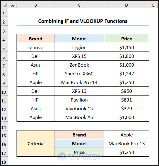
- Output → $1250
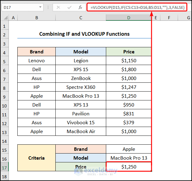
Eventually, your output should look like the following screenshot.
Read More: VLOOKUP with Multiple Criteria Including Date Range in Excel
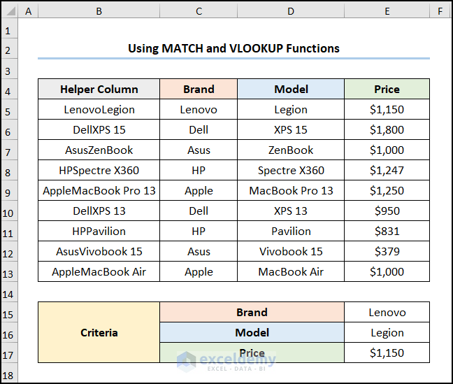
Method-3: Combining VLOOKUP and MATCH Functions
Another way to use VLOOKUP with multiple criteria in different columns involves using the MATCH function. Now, the MATCH function returns the relative position of an item matching a specific value in an array, therefore, let’s see it in action.
📌 Steps:
- First and foremost, create a Helper Column as shown previously >> proceed to the E17 cell >> enter the formula given below.
=VLOOKUP(E15&E16,B5:E13,MATCH(C17,B4:E4,0),FALSE)
In the above expression, the E15 and E16 cells represent the Brand and Model names while the C17 cell indicates the Price and the B4:E4 point to the column headers.
Formula Breakdown:
- MATCH(C17,B4:E4,0) → returns the relative position of an item in an array matching the given value. Here, C17 is the lookup_value argument which refers to the Price. Following, B4:E4 represents the lookup_array argument from where the value is matched. Lately, 0 is the optional match_type argument which indicates the Exact match criteria.
- Output → 4
- VLOOKUP(E15&E16,B5:E13,MATCH(C17,B4:E4,0),FALSE) → becomes
- VLOOKUP(E15&E16,B5:E13, 4, FALSE) → Here, E15&E16 ( lookup_value argument) is mapped from the B5:E13 (table_array argument) array. Next, 4 (col_index_num argument) represents the column number of the lookup value. Lastly, FALSE (range_lookup argument) refers to the Exact match of the lookup value.
- Output → $1150
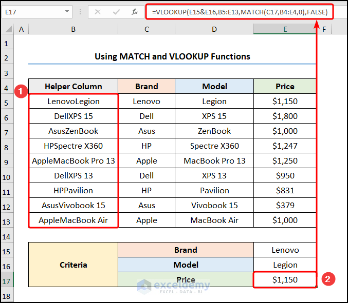
Lastly, the results should look like the image given below.
Method-4: Utilizing VLOOKUP and CHOOSE Functions
If you want to learn about more techniques, you can apply the CHOOSE and VLOOKUP functions to generate a virtual helper column and return a value based on the given criteria. Now, allow me to demonstrate the process in the steps below.
📌 Steps:
- Initially, navigate to the D17 cell >> copy and paste the following expression.
=VLOOKUP($D$15&$D$16,CHOOSE({1,2},$B$5:$B$13&$C$5:$C$13,$D$5:$D$13),2,FALSE)
In this expression, the D15 and D16 cells point to the Brand and Model.
Formula Breakdown:
- CHOOSE({1,2},$B$5:$B$13&$C$5:$C$13,$D$5:$D$13) → chooses a value or action to perform from a list of values, based on an index number. Here, {1,2} is the index_num argument while $B$5:$B$13&$C$5:$C$13, $D$5:$D$13 represents the value1, and value2 arguments. Accordingly, the function combines the Brand and Model names and stores them in the first column and keeps the Price in the second column.
- VLOOKUP($D$15&$D$16,CHOOSE({1,2},$B$5:$B$13&$C$5:$C$13,$D$5:$D$13),2,FALSE) → looks for a value in the left-most column of a table, and then returns a value in the same row from a column you specify. Here, $D$15&$D$16 ( lookup_value argument) is mapped from the CHOOSE({1,2},$B$5:$B$13&$C$5:$C$13,$D$5:$D$13) (table_array argument) array which creates a virtual Helper Column. Next, 2 (col_index_num argument) represents the column number of the lookup value in the virtual Helper Column. Lastly, FALSE (range_lookup argument) refers to the Exact match of the lookup value.
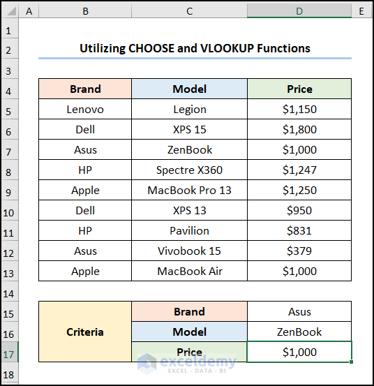
- Output → $1000
📃 Note: Please make sure to use Absolute Cell Reference by pressing the F4 key on your keyboard.
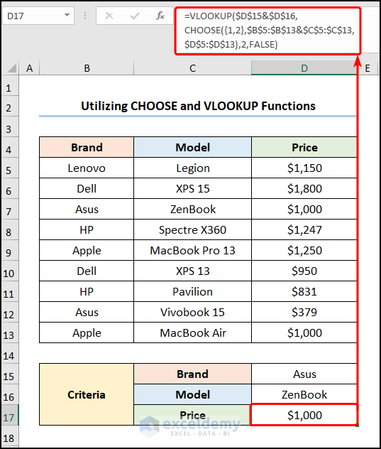
Consequently, the output should look like the screenshot given below.
Read More: How to Apply VLOOKUP with Multiple Criteria Using the CHOOSE Function
Method-5: Applying Drop-Down List with VLOOKUP Function
We can also incorporate Excel’s drop-down lists and use VLOOKUP with multiple criteria in different columns to select the input criteria from the drop-down lists and get the corresponding result. So, follow these simple steps.
📌 Steps:
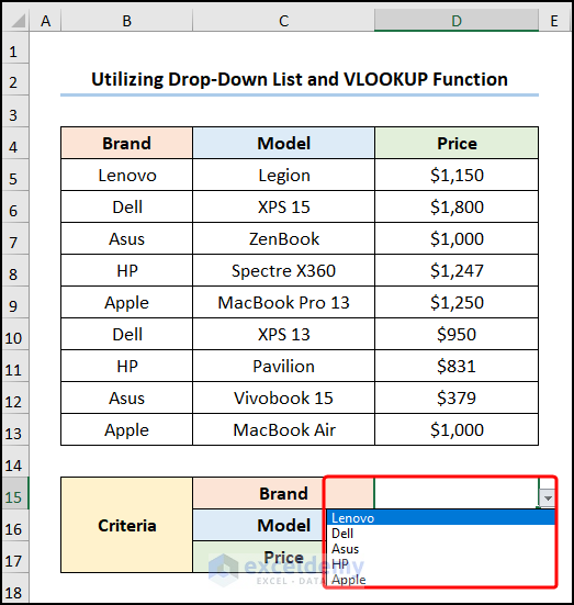
- First, go to the D15 cell >> click the Data tab >> then press the Data Validation drop-down.

This opens the Data Validation dialog box.
- Second, in the Allow drop-down choose the List option >> in the Source field, select the B5:B19 cells with the unique Brand names >> click the OK button.
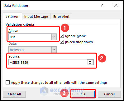
Now, this inserts a drop-down list as shown in the picture below.
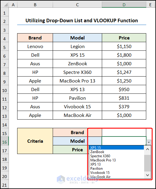
- Similarly, insert another drop-down list for the Model names.
- Third, proceed to the D17 cell >> enter the following expression in the Formula Bar.
=VLOOKUP(D15,IF(C5:C13=D16,B5:D13,""),3,FALSE)
Here, the D15 and D16 cells point to the Brand and Model.
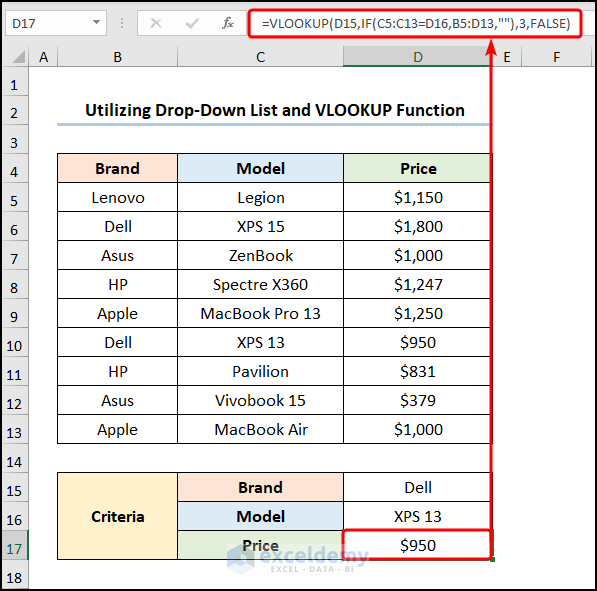
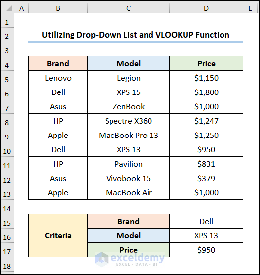
Subsequently, the results should look like the image shown below.
Employing INDEX and MATCH Functions to Lookup a Value
An alternative to the VLOOKUP function is combining the INDEX and MATCH functions which are commonly applied in Excel to look up a value based on certain criteria. So, let’s begin.
📌 Steps:
- To begin with, navigate to the D17 cell and type in the formula given below.
=INDEX(D5:D13,MATCH(1,(B5:B13=D15)*(C5:C13=D16),0))
Here, the B5:B13, C5:C13, and D5:D13 indicate the Brand, Model and Price respectively.
Formula Breakdown:
- MATCH(1,(B5:B13=D15)*(C5:C13=D16),0) → returns the relative position of an item in an array matching the given value. Here, 1 is the lookup_value argument. Following, (B5:B13=D15)*(C5:C13=D16) represents the lookup_array argument from where the value is matched. Lastly, 0 is the optional match_type argument which indicates the Exact match criteria.
- Output → 9
- INDEX(D5:D13,MATCH(1,(B5:B13=D15)*(C5:C13=D16),0)) → becomes
- =INDEX(D5:D13,9) → returns a value at the intersection of a row and column in a given range. In this expression, the D5:D13 is the array argument that represents the Prices. Lastly, 9 is the row_num argument which indicates the row location.
- Output → $1000
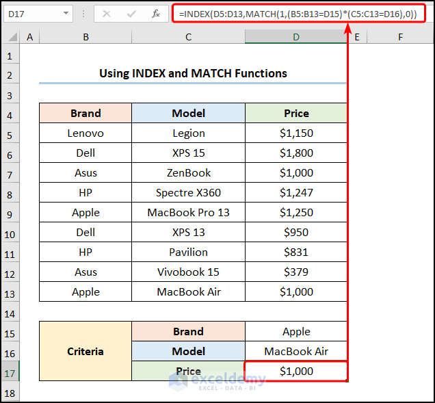
Consequently, your output should look like the picture given below.
Read More:Excel VLOOKUP with Multiple Criteria in Column and Row
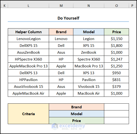
Practice Section
We have provided a Practice section on the right side of each sheet so you can practice yourself. Please make sure to do it by yourself.
Download Practice Workbook
You can download the practice workbook from the link below.
Conclusion
To conclude, I hope this tutorial has provided you with useful knowledge on how to use VLOOKUP with multiple criteria in different columns in Excel. We recommend you learn and apply all these instructions to your dataset. Download the practice workbook and try these yourself. Also, feel free to give feedback in the comment section. Your valuable feedback keeps us motivated to create tutorials like this.
Related Articles
- Excel VLOOKUP with Multiple Criteria in Horizontal & Vertical Way
- Vlookup with Multiple Criteria without a Helper Column in Excel
- How to Use VLOOKUP with Multiple Criteria in Different Sheets
<< Go Back to VLOOKUP with Multiple Criteria | Excel VLOOKUP Function | Excel Functions | Learn Excel
Get FREE Advanced Excel Exercises with Solutions!
