Example of VLOOKUP with Multiple IF Condition in Excel (9 Criteria)

One of the most used functions in Excel is the VLOOKUP function and it’s quite powerful too. We can make it more effective by using the IF function with the VLOOKUP function. We can apply those two functions together to perform various operations. In this article, we will use the example to show you the effectiveness of VLOOKUP with Multiple IF Condition in Excel.

Introduction to Excel VLOOKUP Function

• Syntax

VLOOKUP(lookup_value, table_array, col_index_num, [range_lookup])

• Arguments

lookup_value: The value to look for in the leftmost column of the given table.

table_array: The table in which it looks for the lookup_value in the leftmost column.

col_index_num: The number of the column in the table from which a value is to be returned.

[range_lookup]: Tells whether an exact or partial match of the lookup_value is required. 0 for an exact match, 1 for a partial match. Default is 1 (partial match). This is optional.

Introduction to Excel IF Function

• Syntax

IF(logical_test, [value_if_true], [value_if_false])

• Arguments

logical_test: Tests a logical operation.

[value_if_true]: If the logical operation is true, return this value.

[value_if_false]: If the logical operation is false, return this value.

Example of VLOOKUP with Multiple IF Condition in Excel: 9 Criteria

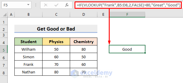
1. Use VLOOKUP with IF Condition to Get Good or Bad

In our first example, we’ll find out if a certain mark obtained by a student is good or bad. Therefore, follow the steps below to perform the task.

STEPS:

• First, select cell F5.
• Then, type the formula:

• Finally, press Enter and it’ll return the result.

🔎 How Does the Formula Work?

• VLOOKUP(“Frank”,B5:D8,2,FALSE)>80

The VLOOKUP function searches for Frank in the range B5:D8 and returns the mark (70) in the 2nd column. Eventually, it tests the mark if it’s greater than 80 or not.

• IF(VLOOKUP(“Frank”,B5:D8,2,FALSE)>80,”Great”,”Good”)

The IF function returns Good as 70 is not greater than 80.

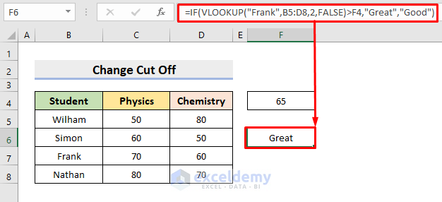
2. Apply VLOOKUP to Change Cut off Value with Multiple IF Condition in Excel

Now, we want to change the cut-off value or want to make it dynamic. Instead of specifying the value in the formula, we’ll place the mark in cell F4. So, learn the steps in this Example to operate VLOOKUP with Multiple IF Condition in Excel.

STEPS:

• Firstly, select cell F6.
• Next, type the formula:

• At last, press Enter.

🔎 How Does the Formula Work?

• VLOOKUP(“Frank”,B5:D8,2,FALSE)>F4

The VLOOKUP function seeks for Frank in the range B5:D8 and returns the mark (70) in the 2nd column. Then, it tests the mark if it’s greater than the F4 cell value (65) or not.

• IF(VLOOKUP(“Frank”,B5:D8,2,FALSE)>F4,”Great”,”Good”)

Finally, The IF function returns Great as 70 is greater than 65.

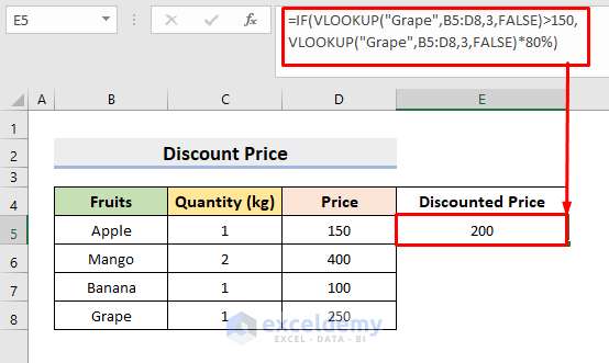
3. Example to Get Discount Price Based on Retail Price with Multiple VLOOKUP & IF Conditions

In the below dataset, we have fixed retail prices for some items. But, we’ll show you how to find out the discounted price with the VLOOKUP & IF functions. Hence, follow the process to know-how.

STEPS:

• In the beginning, select cell E5.
• Afterward, type the formula:

• In the end, press Enter to return the value.

🔎 How Does the Formula Work?

• VLOOKUP(“Grape”,B5:D8,3,FALSE)>150

The VLOOKUP function searches for Grape in the range B5:D8 and returns the price (250) in the 3rd column. Next, it compares the price if it’s greater than 150 or not.

• VLOOKUP(“Grape”,B5:D8,3,FALSE)*80%

This VLOOKUP function searches for Grape in the range B5:D8 and returns the price (250) in the 3rd column. Next, it multiplies the value with .8.

• IF(VLOOKUP(“Grape”,B5:D8,3,FALSE)>150,VLOOKUP(“Grape”,B5:D8,3,FALSE)*80%)

Lastly, the IF function returns VLOOKUP(“Grape”,B5:D8,3,FALSE)*80% output as VLOOKUP(“Grape”,B5:D8,3,FALSE)>150 formula is true.

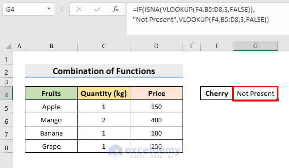
4. Combine Excel VLOOKUP, IF & ISNA Functions with Multiple Conditions

We will look for a certain fruit whether it’s present or not in the dataset and if present, will return the price. Now, learn the Example for performing VLOOKUP with Multiple IF Condition in Excel.

STEPS:

• Select cell G4 at first.
• Then, type the formula:

• Lastly, press Enter.

🔎 How Does the Formula Work?

• VLOOKUP(F4,B5:D8,3,FALSE)

The VLOOKUP function seeks the F4 cell value (Cherry) in the range B5:D8.

• ISNA(VLOOKUP(F4,B5:D8,3,FALSE))

The ISNA function looks for VLOOKUP(F4,B5:D8,3,FALSE) output to see if it’s available or not.

• IF(ISNA(VLOOKUP(F4,B5:D8,3,FALSE)),”Not Present”,VLOOKUP(F4,B5:D8,3,FALSE))

The IF function returns ‘Not Present’ as Cherry is not available in the given dataset.

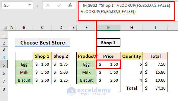
5. Example of Choosing the Best Store with VLOOKUP in Excel

Another use of the VLOOKUP function is that we can compare multiple stores to find out the best deal. Here, we have put Shop 1 in cell G2. Hence, follow the steps to carry out the operation.

STEPS:

• First of all, choose cell G5 to type the formula:

• Subsequently, press Enter and use the AutoFill tool to fill the rest.

🔎 How Does the Formula Work?

• VLOOKUP(F5,B5:D7,2,FALSE)

The VLOOKUP function searches the F5 cell value (Egg) in the range B5:D7 and returns the value ($1.50) in the 2nd column.

• VLOOKUP(F5,B5:D7,3,FALSE)

This VLOOKUP function searches the F5 cell value (Egg) in the range B5:D7 and returns the value ($1.75) in the 3rd column.

• IF($G$2=”Shop 1″,VLOOKUP(F5,B5:D7,2,FALSE),VLOOKUP(F5,B5:D7,3,FALSE))

The IF function compares the G2 cell value (Shop 1) with ‘Shop 1’. As it’s true, the function returns $1.50. If the G2 cell value were Shop 2, it’d have returned $1.75.

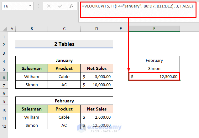
6. VLOOKUP Example with 2 Tables in Excel

So far we have used a single table to fetch data. In this example, we’ll use 2 tables as references. Therefore, learn the following steps of this Example to perform VLOOKUP in 2 Tables with Multiple IF Condition in Excel.

STEPS:

• Select cell F6.
• Type the formula:

• At last, press Enter and it’ll return the Net Sales of Simon.

🔎 How Does the Formula Work?

• IF(F4=”January”, B6:D7, B11:D12)

The IF function compares the F4 cell value (February) with January and returns the range B11:D12 as the logical test is false.

• VLOOKUP(F5, IF(F4=”January”, B6:D7, B11:D12), 3, FALSE)

The VLOOKUP function seeks the F5 cell value (Simon) in the range B11:D12 and returns the Net Sales of $12,500.00 in the 3rd column.

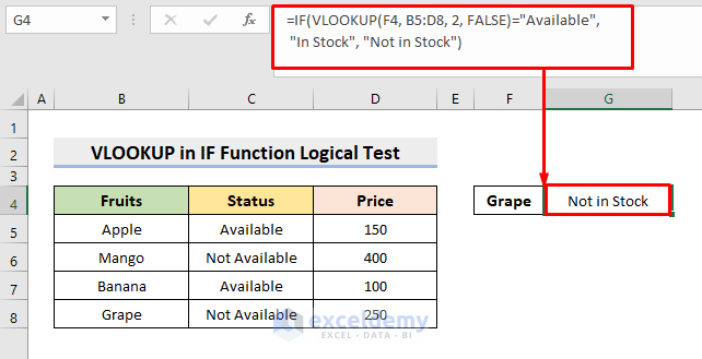
7. Excel VLOOKUP in IF Function Logical Test

Moreover, we can place the VLOOKUP function in the argument section of the IF function. See the following procedure to carry out the operation.

STEPS:

• First of all, choose cell G4 to type the formula:

• Next, press Enter. Thus, you’ll see the output.

🔎 How Does the Formula Work?

• VLOOKUP(F4, B5:D8, 2, FALSE)=”Available”

The VLOOKUP function seeks the F4 cell value (Grape) in the range B5:D8 and compares the value in the 2nd column (Not Available) with Available.

• IF(VLOOKUP(F4, B5:D8, 2, FALSE)=”Available”, “In Stock”, “Not in Stock”)

Finally, the IF function returns Not in Stock as VLOOKUP(F4, B5:D8, 2, FALSE)=”Available” output is false.

Similar Readings

• Excel IF Function with 3 Conditions
• How to Use PERCENTILE with Multiple IF Condition in Excel

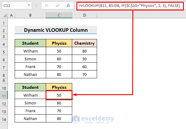
8. Select Column of VLOOKUP Dynamically with IF Function

In this example, we want to create a dynamic column for the VLOOKUP function. For that reason, we’ll make use of the IF function. Hence, go through the below Example to perform VLOOKUP with Multiple IF Condition in Excel.

STEPS:

• In the beginning, select cell C11. Here, type the formula:

• After that, press Enter and it’ll spill the data. Use AutoFill to complete the series.

🔎 How Does the Formula Work?

• IF($C$10=”Physics”, 2, 3)

The IF function compares the C10 cell value (Physics) with Physics as given in the formula. Then, it returns 2 as the logical test is true.

• VLOOKUP(B11, B5:D8, IF($C$10=”Physics”, 2, 3), FALSE)

At last, the VLOOKUP function seeks the B11 cell value (Wilham) in the range B5:D8 and returns the value in the 2nd column (50).

9. Example to Apply VLOOKUP for Dates with Multiple IF Condition in Excel

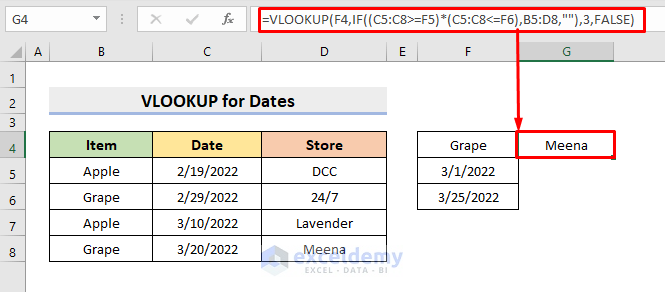
Additionally, we can apply VLOOKUP for dates. So, learn the steps of this Example to apply VLOOKUP for Dates with Multiple IF Condition in Excel.

STEPS:

• Click cell G4.
• Type the formula:

• Lastly, press Enter.

🔎 How Does the Formula Work?

• IF((C5:C8>=F5)*(C5:C8<=F6),B5:D8,””)

The IF function compares each cell of the range C5:C8 with F5 and F6 cell values. Subsequently, it returns the range B5:D8 as the logical test is true.

• VLOOKUP(F4,IF((C5:C8>=F5)*(C5:C8<=F6),B5:D8,””),3,FALSE)

Finally, the VLOOKUP function seeks the F4 cell value (Grape) in the range B5:D8 and returns the value in the 3rd column (Meena).

Alternative Example of VLOOKUP with Multiple IF Condition in Excel

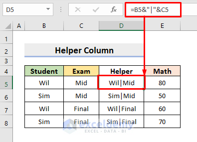
1. Helper Column for Multiple Criteria in Excel

We can create a helper column for multiple criteria in Excel. Therefore, follow the steps to insert a helper column.

STEPS:

• First, select cell D5.
• Then, type the formula:

• After that, press Enter and it’ll return the value. Use AutoFill to fill the series.

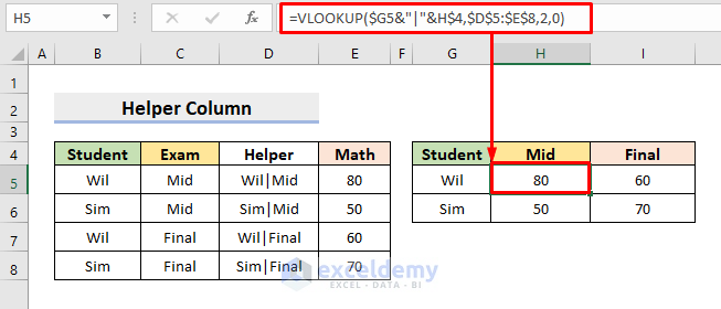
• Subsequently, select cell H5 to type the formula:

• Press Enter and use AutoFill to complete the rest.

Here, the VLOOKUP function looks for the $G5&”|”&H$4 cell value (Wil|Mid) in the range $D$5:$E$8 and it returns 80 present in the 2nd column.

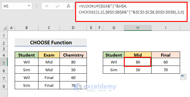
2. Multiple Criteria Example with CHOOSE Function

We’ll use the CHOOSE function along with VLOOKUP in this example to avoid the helper column. Learn the process to carry out the operation.

STEPS:

• Firstly, select cell H5.
• Next, type the formula:

• At last, press Enter and it’ll return the value.

🔎 How Does the Formula Work?

• CHOOSE({1,2},$B$5:$B$8&”|”&$C$5:$C$8,$D$5:$D$8)

The CHOOSE function spills B5:D8 data into 2 columns merging the cell values in the B and C columns together.

• VLOOKUP($G5&”|”&H$4,CHOOSE({1,2},$B$5:$B$8&”|”&$C$5:$C$8,$D$5:$D$8),2,0)

The VLOOKUP function searches for $G5&”|”&H$4 in the range B5:D8 and returns 80 present in the 2nd column.

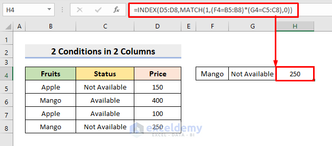
3. VLOOKUP Function with Two Conditions in Two Columns

Instead of using VLOOKUP, we can use the INDEX MATCH formula to pull the data based on 2 conditions in 2 separate columns. Hence, follow the procedure to perform the task.

STEPS:

• In the beginning, select cell H4.
• Afterward, type the formula:

• In the end, press Enter to return the value.

🔎 How Does the Formula Work?

• MATCH(1,(F4=B5:B8)*(G4=C5:C8),0)

The MATCH formula returns 4 to INDEX as the row number. Here, we compare the multiple criteria by applying boolean logic.

• INDEX(D5:D8,MATCH(1,(F4=B5:B8)*(G4=C5:C8),0))

Lastly, the INDEX function returns 250 which is in the 4th row in the range D5:D10.

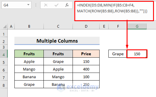
4. VLOOKUP for Multiple Columns in Excel

We’ll apply the INDEX MATCH formula for performing the lookup operation in multiple columns and returning the Price of the mentioned fruit. So, learn the steps below.

STEPS:

• Select cell G4 at first.
• Then, type the formula:

• Lastly, press Enter.

🔎 How Does the Formula Work?

• ROW(B5:B8)

First, the ROW function returns the respective row numbers.

• MATCH(ROW(B5:B8),ROW(B5:B8))

Then, the MATCH formula outputs are 1, 2, 3, and 4.

• IF(B5:C8=F4,MATCH(ROW(B5:B8),ROW(B5:B8)),””)

The IF function compares each cell in B5:C8 with the F4 cell value and returns the values where it finds TRUE for the logical test.

• MIN(IF(B5:C8=F4,MATCH(ROW(B5:B8),ROW(B5:B8)),””))

The MIN function returns the smallest value (1) out of the IF(B5:C8=F4,MATCH(ROW(B5:B8),ROW(B5:B8)),””) outputs.

• INDEX(D5:D8,MIN(IF(B5:C8=F4,MATCH(ROW(B5:B8),ROW(B5:B8)),””)))

Eventually, the INDEX function returns 150 which is in the 1st row in the range D5:D8.

Download Practice Workbook

Download the following workbook to practice by yourself.

Conclusion

Henceforth, you will be able to operate VLOOKUP with Multiple IF Conditions in Excel as shown in the examples. Keep using them and let us know if you have any more ways to do the task. Don’t forget to drop comments, suggestions, or queries if you have any in the comment section below.