How to Use PERCENTILE with Multiple IF Condition in Excel (3 Examples)

Excel PERCENTILE Function Introduction

In Excel, the PERCENTILE function is used to compute the k-th percentile of values in a range or array. For example, you can easily compute students who score above the 80-th percentile. Excel has introduced alternatives to the PERCENTILE function in the newer versions for a more accurate result.

• Syntax

PERCENTILE(array,k)

• Arguments

array: This is the first required argument. It is the range from where the percentile needs to be calculated.

k: The second argument denotes the k-th percentile. If you want to calculate 90-th percentile, then you need to type 90 in place of k.

Excel IF Function Introduction

The IF function checks a criterion or condition. Then, it returns one value if it is TRUE or another value if it is FALSE.

• Syntax

IF(logical_test,[value_if_true],[value_if_false])

• Arguments

logical_test: This is the first and compulsory argument. Here, you need to enter the condition that you want to check.

[value_if_true]: It is an optional argument. In this argument, you need to type the value that your formula should return if the condition is TRUE.

[value_if_false]: Here, you need to enter the value that the formula should return if the condition is FALSE.

How to Use PERCENTILE with Multiple IF Conditions in Excel: 3 Examples

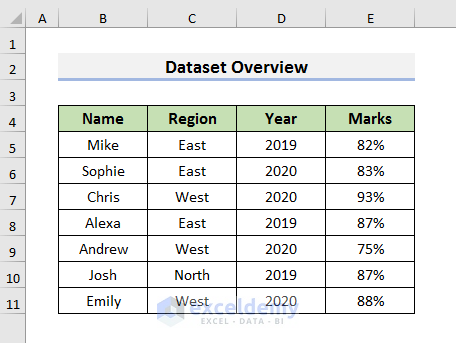
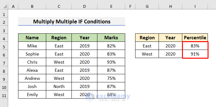
We will use a dataset that contains information about the Marks obtained by some students on a test. The students are from different regions and the test was held in different years. We will try to use multiple conditions to calculate the percentile in the following examples.

Method 1 – Multiplying IF Conditions Inside the Excel PERCENTILE Function

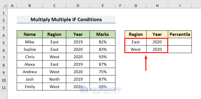
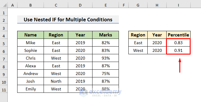
We will calculate the percentile based on two conditions. We will show the percentile of the East region in the 2020 year in Cell I5 and the West region in the 2020 year in Cell I6.

Steps:

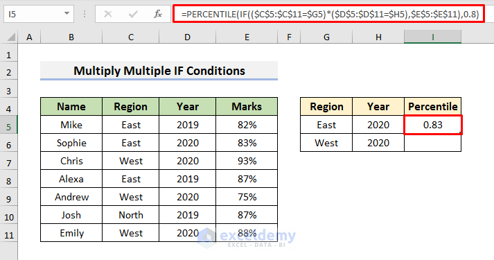
• Select Cell I5 and insert this formula:

• Hit Enter to see the result.

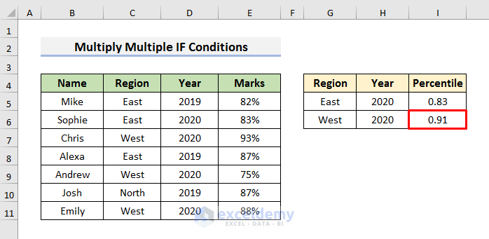
• Drag the Fill Handle down to see the result in Cell I6.

• Select Cells I5 and I6.
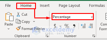
• Go to the Home tab and select Percentage from the Number field.

• You will see the percentages.

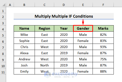
• If you want to add more conditions, you need to add the condition in the formula by multiplying. We have added Gender as another condition in Column E.

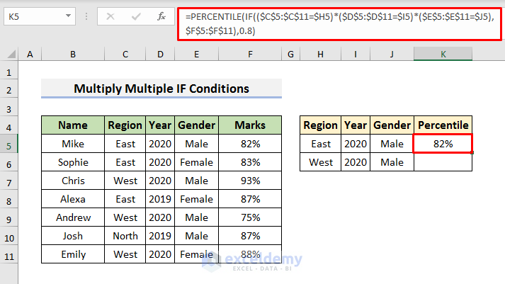
• To add the condition, multiply it like the formula below:

• Press Enter to see the result.

How Does the Formula Work?

• ($C$5:$C$11=$H5)

This is the first condition and it denotes that the Region will have to be the East.

• ($D$5:$D$11=$I5)

It is the second condition and represents that the Year will have to be 2020.

• ($E$5:$E$11=$J5)

This is the third condition and denotes that the Gender will have to be Male.

• IF(($C$5:$C$11=$H5)*($D$5:$D$11=$I5)*($E$5:$E$11=$J5),$F$5:$F$11)

Here, the IF function contains multiple conditions in the first argument and the range of values in the second argument. We have multiplied the conditions to get our desired result. The range of values is the obtained Marks.

• PERCENTILE(IF(($C$5:$C$11=$H5)*($D$5:$D$11=$I5)*($E$5:$E$11=$J5),$F$5:$F$11),0.8)

This formula calculates the 80-th percentile. That is why we have entered 0.8 in the second argument. It will provide the result if all the conditions are satisfied.

Read More: Excel IF Function with 3 Conditions

Method 2 – Use a Nested IF to Apply Multiple Conditions Inside the PERCENTILE Function in Excel

Steps:

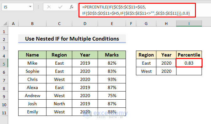
• Select Cell I5 and insert this formula:

• Hit Enter to see the result.

• Use the Fill Handle to see the result in Cell I6.

• Select the cells.
• Go to the Home tab and select Percentage in the Number section.

• You will see results like the picture below.

How Does the Formula Work?

• IF($E$5:$E$11<>””,$E$5:$E$11)

This formula denotes that the Range of values is E5:E11.

• IF($D$5:$D$11=$H5,IF($E$5:$E$11<>””,$E$5:$E$11)

Here, the formula contains the condition of the Year and a nested IF of the Range of values.

• IF($C$5:$C$11=$G5,IF($D$5:$D$11=$H5,IF($E$5:$E$11<>””,$E$5:$E$11))

This formula contains the condition of the Region and nested IF formulas that denote the Year and the Range of values. In this case, the formula will check whether the region is East, then, the year is 2020, and then the Marks.

• PERCENTILE(IF($C$5:$C$11=$G5,IF($D$5:$D$11=$H5,IF($E$5:$E$11<>””,$E$5:$E$11))),0.8)

The PERCENTILE function computes the 80-th percentile. That is why we have entered 0.8 in the second argument. It will provide the result if all the conditions are satisfied.

Read More: Example of VLOOKUP with Multiple IF Condition in Excel

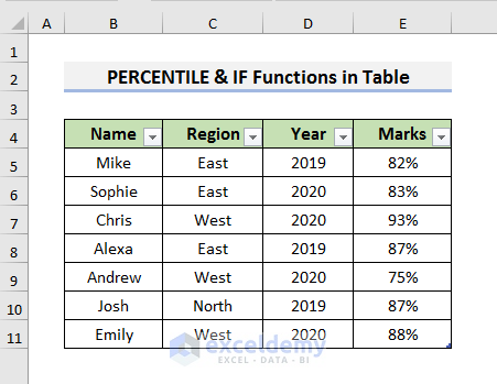
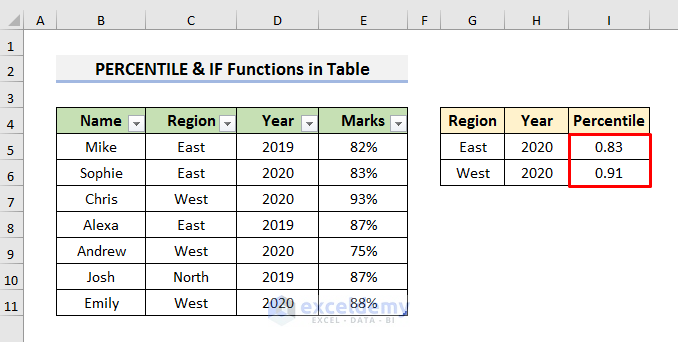
Method 3 – Combine PERCENTILE and IF Functions with Multiple Condition in Excel Table

The previous dataset is converted into a table. We will calculate the percentile based on two conditions.

Steps:

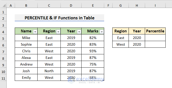
• Create the structure to see the percentile like in the picture below.

• Select Cell I5 and insert this formula:

• Press Enter to see the result.

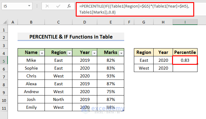
This formula will calculate the percentile if the region is East and the year is 2020. This formula works the same as the formula in Method 1. We are using two conditions. The representation is different because we are applying this formula in a table.

• Drag down the Fill Handle to see the result in Cell I6.

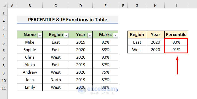
• To convert the numbers into percentages, select Percentage in the Number field from the Home tab.

• You will see results like the image below.

How Does the Formula Work?

• Table1[Region]=$G5

This is the first condition and it means the region will have to be East.

• Table1[Year]=$H5

It is the second condition and means the year will have to be 2020.

• IF((Table1[Region]=$G5)*(Table1[Year]=$H5),Table1[Marks])

This formula multiplies the conditions in the first argument and the range of marks in the second argument. The multiplication of the conditions means all conditions must be fulfilled to get the result.

• PERCENTILE(IF((Table1[Region]=$G5)*(Table1[Year]=$H5),Table1[Marks]),0.8)

The formula calculates the 80-th percentile in a table named Table1.

Things to Remember

Here, we have used an array formula in the above methods. If the formula doesn’t work after pressing Enter, then you need to press Ctrl + Shift + Enter.

Download the Practice Book

<< Go Back to Multiple IF Condition in Excel | Excel IF Function | Excel Functions | Learn Excel