This is an overview.
The INDEX and the MATCH Functions in Excel
The INDEX function returns a value or a reference to a value from a table or range of values.
Syntax:
=INDEX (array, row_num, [column_num])
- array: The range of cells from which data will be retrieved; Required.
- row_num: The reference row number from which data should be returned.
- column_num: The reference column number from which data should be returned.
The MATCH function searches for a specified value in a range of cells and then returns the position of that value in that range.
Syntax:
MATCH(lookup_value,lookup_array,[match_type])
- lookup_value: The value that you want to match in the range of cells.
- lookup_array: The range of cells from which it’ll search for the lookup_value.
- [match_type]: Here, 1= the value is less than the exact match, 0= the Exact match, -1= the value is greater than the exact match.
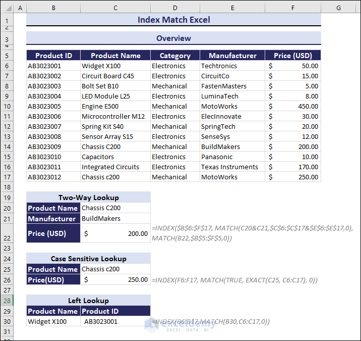
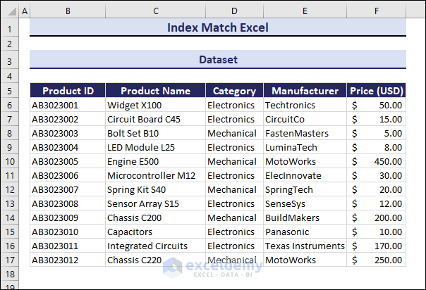
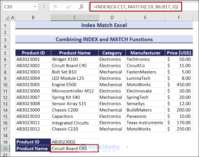
The sample dataset includes details of mechanical and electrical products (Product ID, Product Name, Category, Manufacturer, and Price).
How to Combine the INDEX and the MATCH Functions in Excel
Using the Product ID, you will search for the Product Name:
- Enter this formula in C20.
=INDEX(C6:C17, MATCH(C19, B6:B17, 0))Product Name is Circuit Board C45.
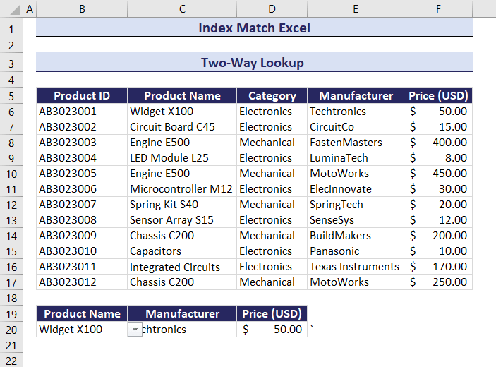
Example 1 – Two-Way Lookup Using the INDEX and the MATCH Functions
Use the Product Name and Manufacturer columns to find the Price of a product:
- Enter the following formula in D20.
=INDEX($B$6:$F$17, MATCH(B20&C20,$C$6:$C$17&$E$6:$E$17,0), MATCH(D19,$B$5:$F$5,0))The formula returns the Price of the given Product Name and Manufacturer: $50.00.
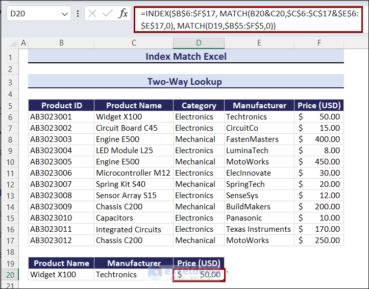
Observe the GIF. Price changed after changing the value of the Product Name and the Manufacturer.
Example 2 – Lookup Value Based on Multiple Criteria Using the INDEX MATCH Function
Three criteria were used: Category, Product Name, and Manufacturer. To search for the Price of the product:
- Enter the following formula in E20.
=INDEX(F6:F17,MATCH(B20&C20&D20,D6:D17&C6:C17&E6:E17,0))The price is $50.00.
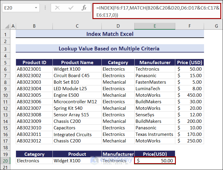
If you change the criteria, the price will also change. Observe the GIF below.
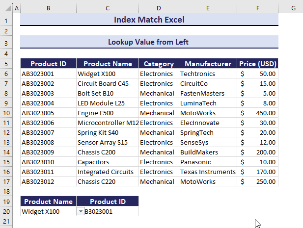
Example 3 – Lookup a Value from the Left in Excel
Look for Product ID by using the column Product Name:
- Select C20.
- Enter the following formula, and press Enter.
=INDEX(B6:B17,MATCH(B20,C6:C17,0))You will find the Product ID: AB3023001.
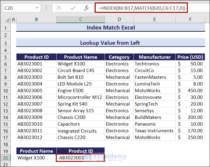
If you change the value in Product Name, Product ID will also change.
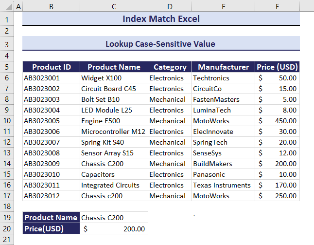
Example 4 – Lookup a Case-Sensitive Value Using the INDEX and the MATCH functions
- Use the formula in C20.
=INDEX(F6:F17, MATCH(TRUE, EXACT(C19, C6:C17), 0))You will get the Price: $200.00.
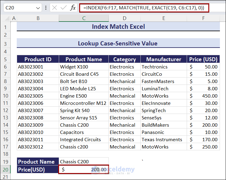
Observe the GIF. C200 was changed to c200. The corresponding value also changed.
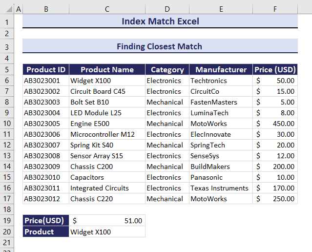
Example 5. Finding the Closest Match Using the INDEX and the MATCH functions
To find the Product Name of the closest match to Price: $51.00:
- Use the formula in C20.
=INDEX(C6:C17, MATCH(MIN(ABS(F6:F17-C19)), ABS(F6:F17-C19), 0))The Price of Widget X100 is $50.00, which is the closest to $51.00.
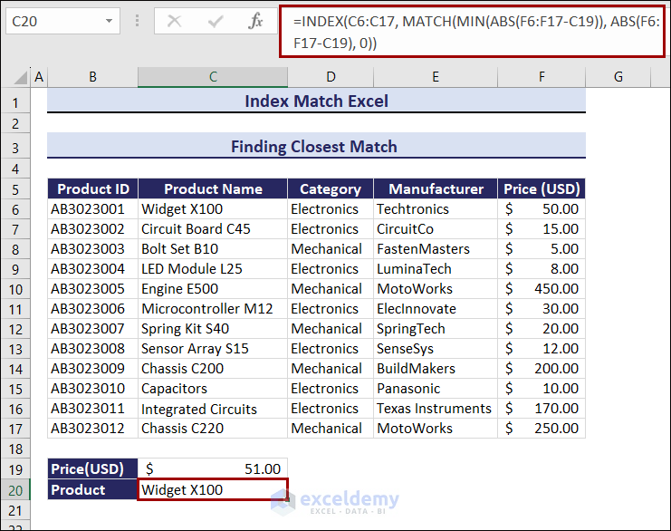
If you change the Price, Product Name will change. Observe the GIF below.
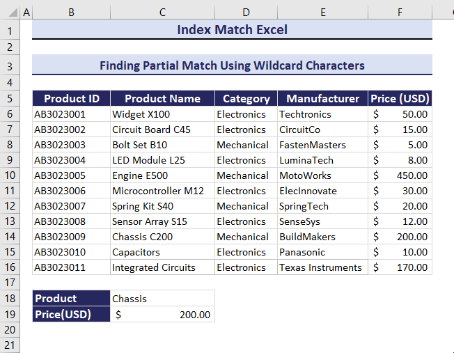
Example 6 – Finding Partial Matched Data Using Wildcard Characters in the INDEX and in the MATCH Formula
Enter the partial Product Name (Chassis instead of Chassis C200) to extract the Price:
- Select C19 and enter the following formula:
=INDEX($F$6:$F$16,MATCH($C$18&"*",$C$6:$C$16,0))The Price of Chassis C200 is $200.00.
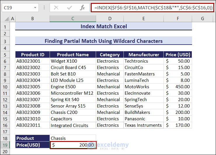
Change the lookup value for the partial match and the outcome will change. Observe the GIF.
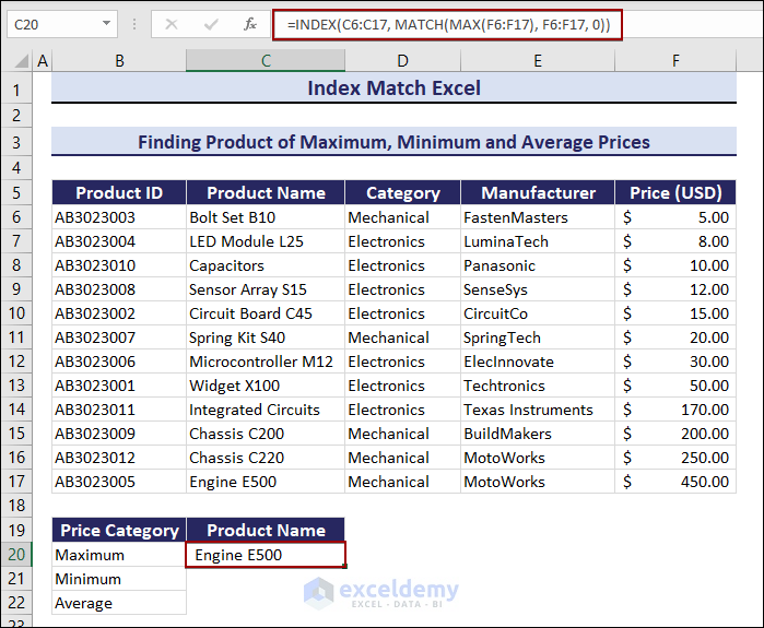
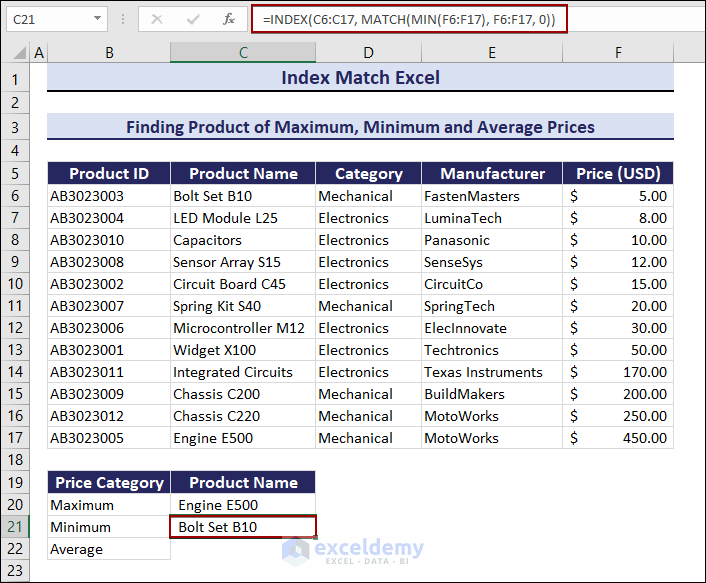
Example 7 – Find the Minimum, Maximum, and Average Values Using the INDEX and the MATCH functions
- Select C20 and enter the formula below.
=INDEX(C6:C17, MATCH(MAX(F6:F17), F6:F17, 0))Engine E500 is the product with the Maximum price.
Find the minimum price of the product:
- Enter the following formula in C21.
=INDEX(C6:C17, MATCH(MIN(F6:F17), F6:F17, 0))Bolt Set B10 is the product with the Minimum price.
To find the closest average value:
- Enter the following formula in C22 and press Enter.
=INDEX(C6:C17, MATCH(AVERAGE(F6:F17), F6:F17,1))The item with the closest average price is the Widget X100.
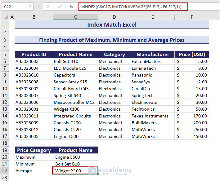
Note:
- You can enter 0 for the exact match. No sorting is required If the value in your lookup array is exactly the average.
- Add 1 to the formula if your lookup column is ordered in ascending order. The formula will find the greatest value that is less than or equal to the average value.
- Enter -1 if your lookup column is arranged in descending order. The formula will find the least value greater than or equal to the average value.
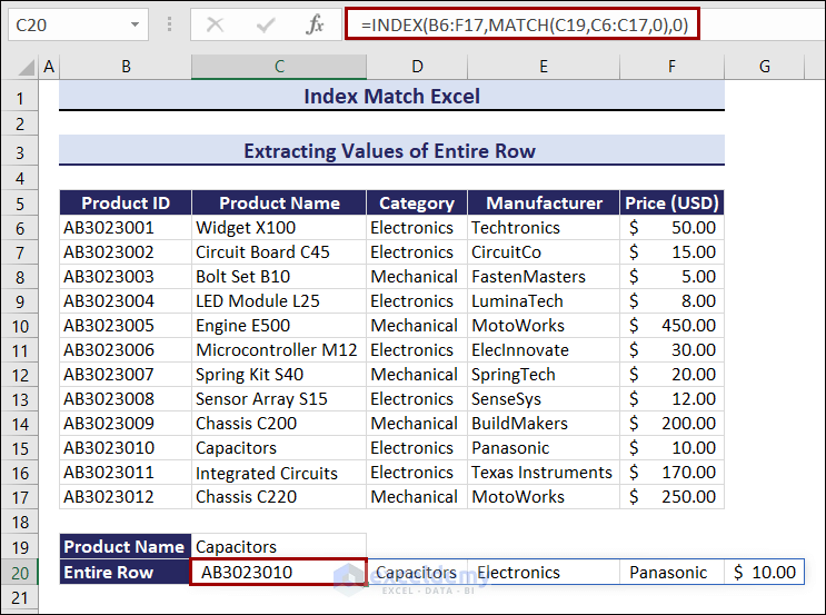
Example 8 – Extract Values of Entire Rows with the INDEX and the MATCH Formulas
To extract the entire row by defining the Product Name:
- Enter the following formula in C20.
=INDEX(B6:F17,MATCH(C19,C6:C17,0),0)You will get the full row for Capacitors.
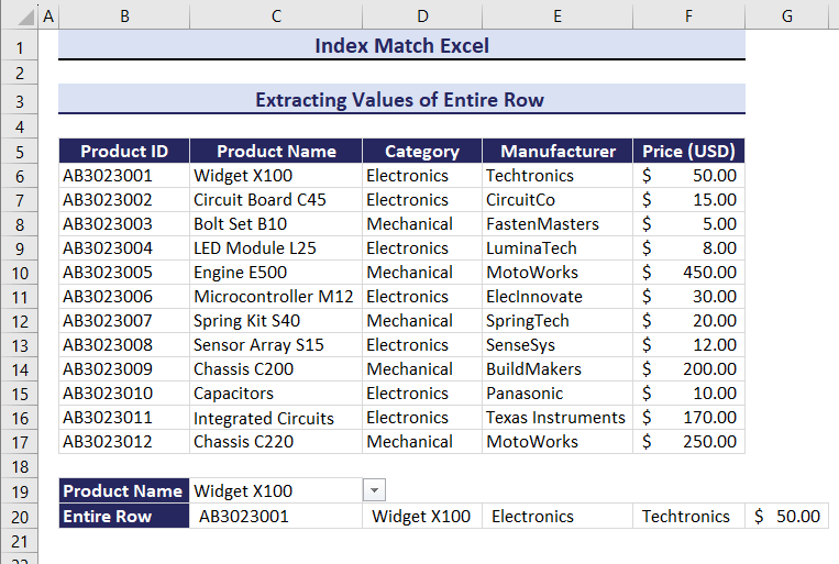
Change the Product Name and the entire row changes. Observe the GIF below.
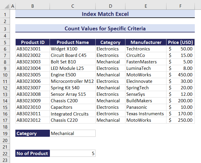
Example 9 – Count Values for Specific Criteria Combining the INDEX, MATCH and COUNTIF Functions
To count the number of products in the Electronics or Mechanical categories:
- Enter the following formula in C22.
=COUNTIF(INDEX($B$6:$F$17,0,MATCH(B19,$B$5:$F$5,0)),C19)The total number of products in the Mechanical category is 5.
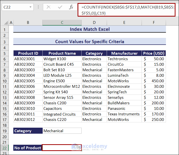
If you change the category from Mechanical to Electronics, the outcome will change. The result is 7. Observe the GIF below.
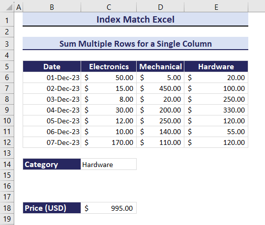
Example 10- Sum Multiple Rows for a Single Criteria
To calculate the total price based on the three columns: Electronics, Mechanical, and Hardware:
- Enter the following formula in C18.
=SUM(INDEX(B6:E12, 0, MATCH(C14,B5:E5,0)))The total Price of Electronics is $295.
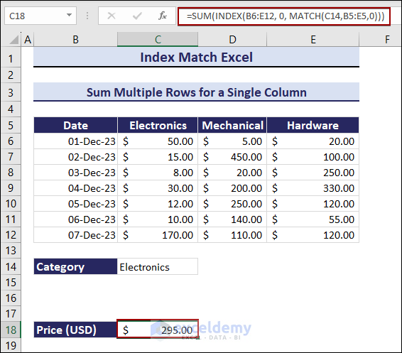
Get the total Price of products in different categories by changing the category in C14. Observe the GIF below.
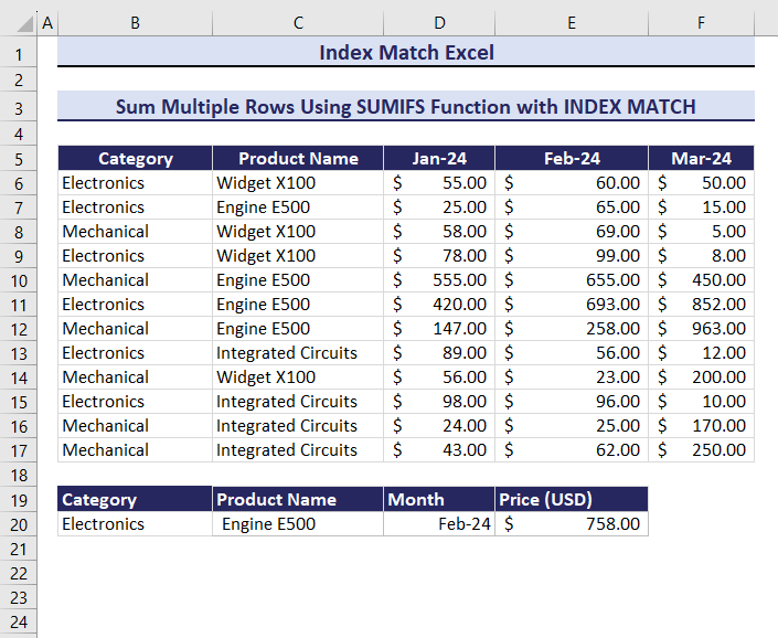
Example 11 – Sum Multiple Rows for Multiple Criteria
To calculate the total Price defining three criteria: Category, Product Name, and Month:
- Enter the following formula in E20.
=SUMIFS(INDEX($D$6:$F$17,,MATCH($D$20,$D$5:$F$5,0)),B6:B17,$B$20,$C$6:$C$17,$C$20)The output is $913.00.
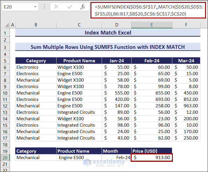
By changing the multiple criteria, the product price will change.
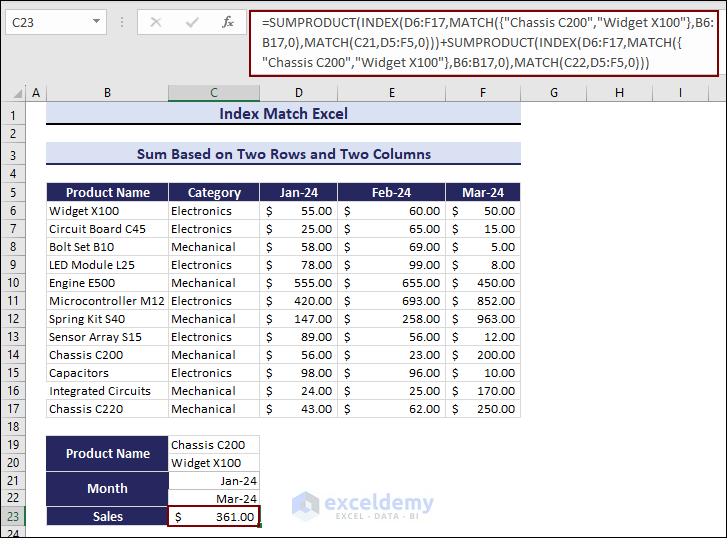
Example 12 – Calculating the Sum Based on Multiple Rows and Multiple Columns
To look for the total sales of Chassis C200 and Widget X100 based on the dates Jan-24 and Mar-24:
- Enter the following formula in C23.
=SUMPRODUCT(INDEX(D6:F17,MATCH({"Chassis C200","Widget X100"},B6:B17,0),MATCH(C21,D5:F5,0)))+SUMPRODUCT(INDEX(D6:F17,MATCH({"Chassis C200","Widget X100"},B6:B17,0),MATCH(C22,D5:F5,0)))The total sales amount is $361.00.
Example 13. Apply the INDEX and the MATCH Formula Across Multiple Sheets
To get the Sales data from different worksheets:
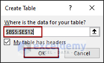
- Select the dataset (B5:E12) >> Go to the Home tab.
- In Styles, select Format as Table.
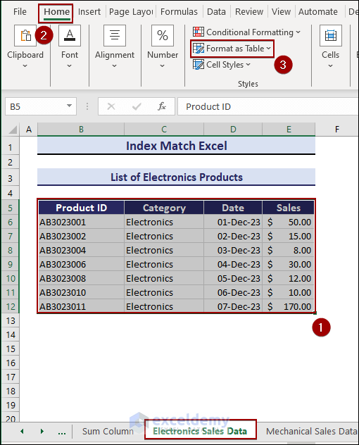
- In the Create Table window, check My table has headers.
- Ckick OK.
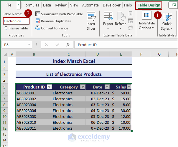
- Choose a color that.
- Click Table Design.
- Change the Table Name to Electronics.
Create tables for the other worksheets: Mechanical Sales Data and Hardware Sales Data.
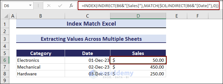
- Create a new sheet and name it (here, Summary). Format the sheet.
- Select D6 in the Summary sheet and enter the following formula:
=INDEX(INDIRECT(B6&"[Sales]"),MATCH($C6,INDIRECT(B6&"[Date]"),0))The Sales for the Electronics category on 01-Dec-23 is $50.00.
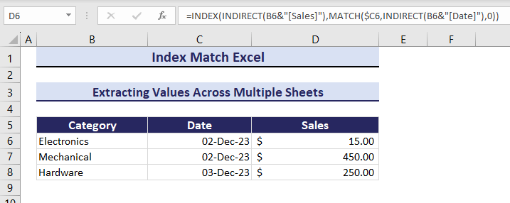
The sales value will change whenever if you modify a category’s date. Observe the GIF below.
Example 14. Finding Duplicate Values in Excel with the INDEX, MATCH, IF, and COUNTIF Functions
- Select E6.
- Enter the following in E6 and press ENTER.
=IF(COUNTIF($D$6:D7,D6)>1,"Duplicate of "&INDEX($C$6:C7,MATCH(D6,$D$6:D7,0)),"Original")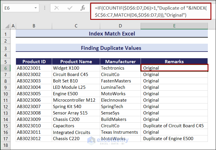
- Use the Fill Handle to find other duplicate values in the dataset.
Alternatives to the INDEX and the MATCH functions in Excel
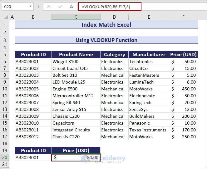
1. Use the VLOOKUP Function
To extract the price of a product using the column number:
- Select B20.
- Enter the following formula and press Enter.
=VLOOKUP(B20,B6:F17,5)The formula will return the Price – $50, for Product ID no. AB3023001.
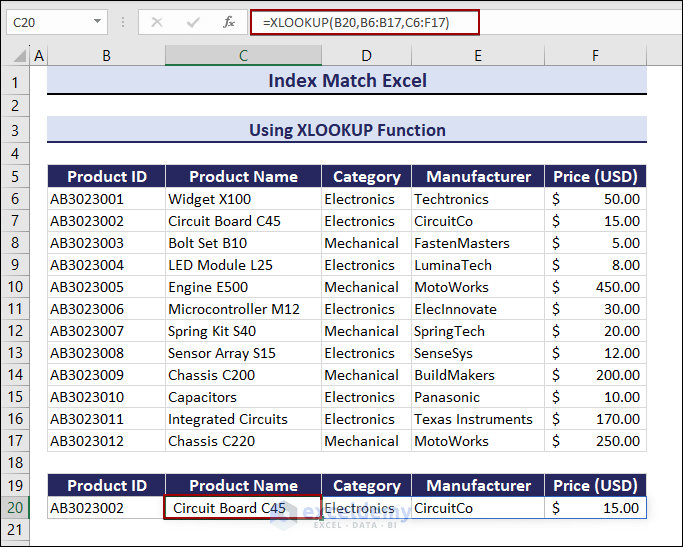
2. Use XLOOKUP Function
To find the Product ID and the entire row of the defined Product ID:
- Select C20 and enter the following formula:
=XLOOKUP(B20,B6:B17,C6:F17)The lookup value is AB3023002. The complete row of that specific cell will be returned by the formula.
Download Practice Workbook
Download the workbook here.
INDEX and MATCH Functions: Knowledge Hub
- Use INDIRECT, INDEX, and MATCH Functions
- XLOOKUP vs INDEX-MATCH
- [Fixed!] INDEX MATCH Not Returning Correct Value
- INDEX MATCH Formulas with Returning Multiple Matches
- INDEX-MATCH Formula to Return Multiple Values Horizontally
- Use IF with INDEX & MATCH Functions
- Sum Multiple Rows Using INDEX MATCH Formula
<< Go Back to Formula List | Learn Excel
Get FREE Advanced Excel Exercises with Solutions!

How to Use INDEX MATCH Formula in Excel (9 Examples) – Problems encountered
1) Step #7 contains three (3) months your solution contains ONLY two (2) months- What about March
2) Step #8 DOES NOT WORK – when you type a formula into A (ONE) cell the results will NOT populate 2 cells to the right. What is the formula utilized to obtain the data within the 2nd & 3rd cell????????? Does this formula only work in a particular Excel Version? 365?? Also, the only way I could get the function to work for the “Salesman” – Frank response was to utilized Ctrl + Shift + Enter Correct???????????????/ If the user needs to utilize Ctrl + Shift + Enter – Would be great if you ADVISED us of this necessity
Dear Rich Saunders,
Query 1: The method 7 works just fine. If you write March in F4, you will get the values for that month as well.
Query 2: The formula is universal for any Excel version. If you write the formula in any cell the formula will get you the entire row value for the name you will write in the F4 cell. For example, if you write “Nathan” in F4 cell and paste the formula in the A1 cell then the formula will write the values of the entire row( B8:D8) in the A1:A3 range.
Yes, we should have mentioned the Ctrl+Shift+Enter in the article. We will make sure of that in the next articles. As we used Microsoft 365 so it works by pressing Enter. We are sorry for that.
Regards
ExcelDemy