Excel INDEX MATCH Formulas with Returning Multiple Matches

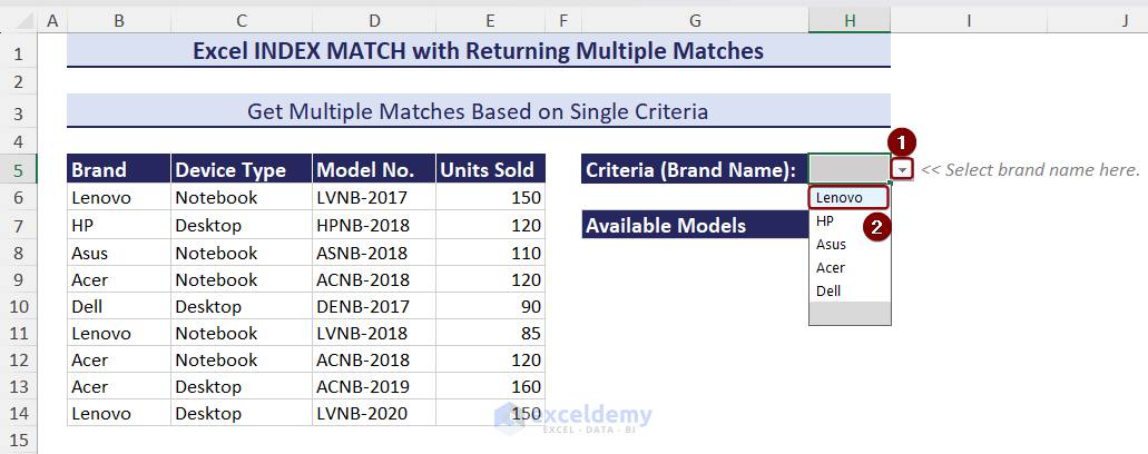
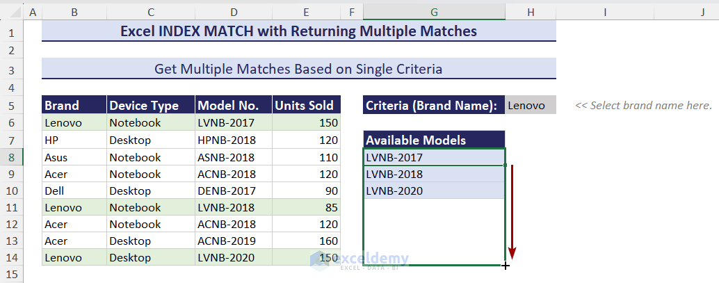
Here we have a sales dataset consisting of the following columns:  Brand, Device Type, Model No. and Units Sold. We want to get all results from the Model No. column based on criteria (brand name) in cell H5.

⏷ Getting Multiple Matches from a Column for Single or Multiple Criteria
⏷ Get Multiple Matches When the Matching Values Contain Duplicates
⏷ Get Multiple Matches from 2 Lookup Array
⏷ Get All Partial Matches

How Does the INDEX-MATCH Combo Work?

INDEX and MATCH functions are used to look up a value in a range of cells and return the corresponding value.

For example, look at the following image– here we have a sales dataset. Say, our lookup value is a brand name: HP and we want to know its sales quantity. So, the lookup array for the MATCH function is B4:B12 (the brand names lie here). The array for the INDEX function is C4:C12 (sales quantity data lie here).

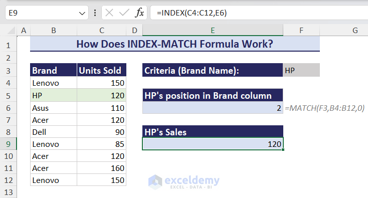
=MATCH("HP",B4:B12,0); this will return 2, as the relative position of HP is 2 in range B4:B12. Here, the last 0 denotes the exact match.

Now, if you write =INDEX(C4:C12,MATCH("HP",B4:B12,0)) inside a cell, it is the same as writing =INDEX(C4:C12,2). So, this formula will return the value from cell C5 (cell number 2 in range C4:C12)

Method 1 – Getting Multiple Matches from a Column with INDEX MATCH Formula for Single or Multiple Criteria

Case 1.1 Returning Multiple Matches for Single Criterion

From the dataset below, we want to get all the model numbers of the Lenovo brand.

Follow the steps below:

• In cell H5, input the brand name ‘Lenovo’.

• Insert the following formula on cell G8:

Here, we have added the IFERROR function in the formula. So, if the main formula finds no match and hence returns #N/A, IFERROR returns an empty string instead of #N/A errors.

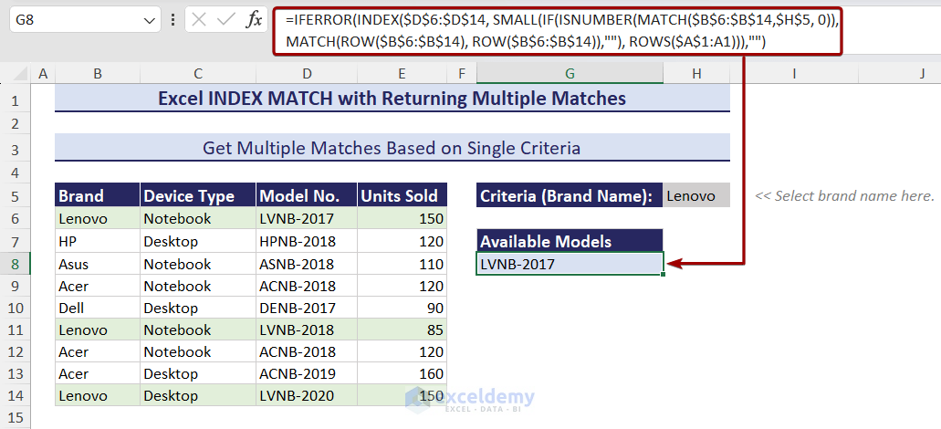
• Drag the Fill Handle icon down until you get blank cells.

Note:

To get the matches horizontally, insert the following formula in cell G9:

Drag the Fill Handle icon to the right.

Alternative Formula (Applicable in Excel 2010 and Later)

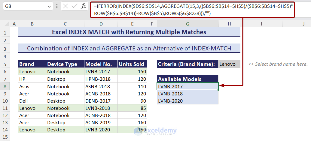
Case 1.2 Returning Multiple Matches for Multiple Criteria

Say, we want to get the model numbers of Lenovo notebooks.

Follow the steps below:

• In cell H5, select the brand name Lenovo.
• In cell H6, write Notebook.

• Insert the following formula on cell G9 and drag the formula down until you get blank cells.

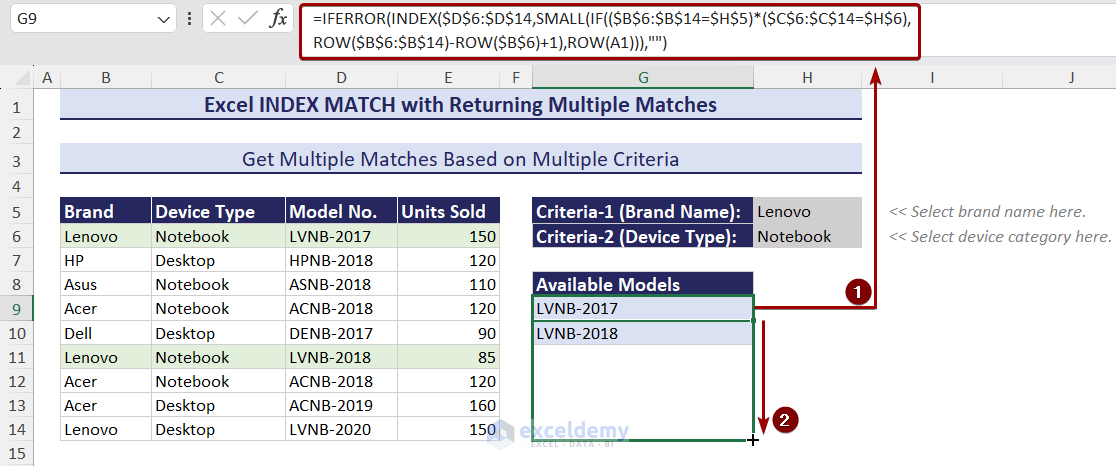
Look at the GIF below. Here, you will see how the matches change with the change in criteria automatically.

Notes:

• You have to set both criteria to get any match using this formula. Only one criterion will not return anything.
• If you want to get the matches in a horizontal manner, use the following formula in cell G9 and drag the Fill Handle to the right:

Easier Alternative Formula for Excel 2019 or Later:

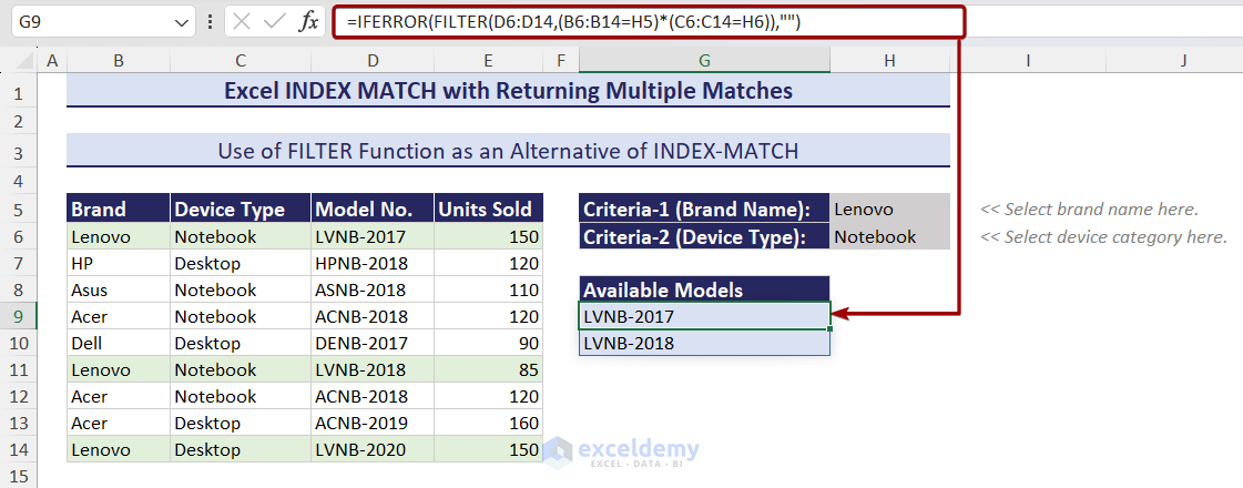
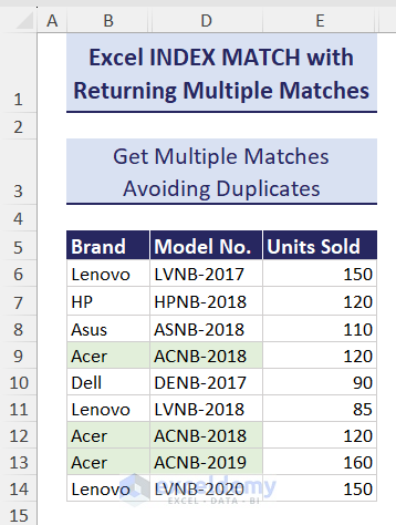
Method 2 – Formula to Get Multiple Matches When the Matching Values Contain Duplicates

In the following data, “Acer ACNB-2018” occurs twice. So, the previous formulas we have shown in Section 1 will return Acer ACNB-2018 twice.

In the main data, Acer is recorded three times, but two of those are the same. If I input the following formula, I get the wrong output:

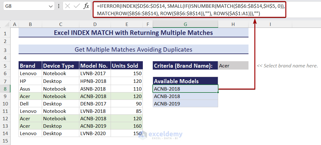
But if I use the following formula inside cell G8 to get all matches for Acer – avoiding duplicates – I get correct outputs.

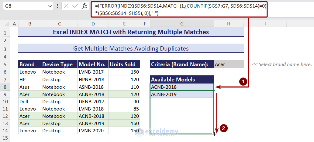
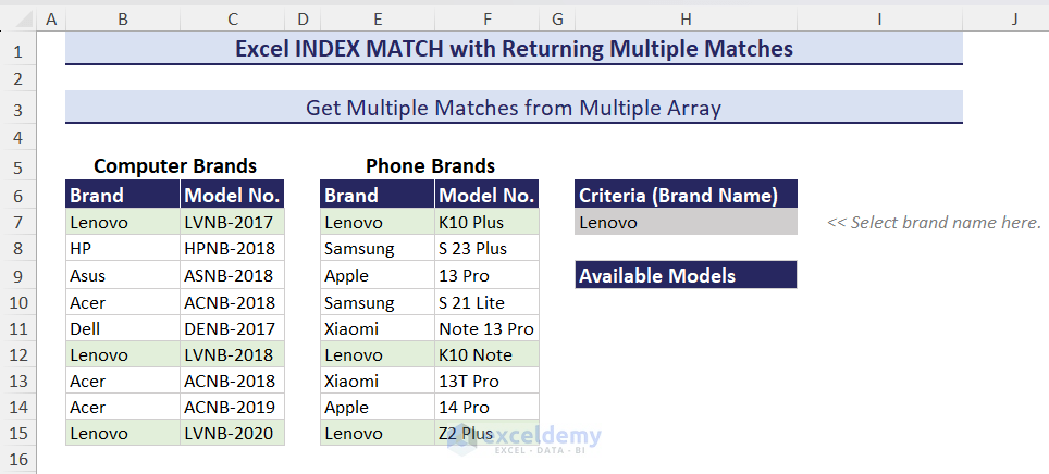
Method 3 – INDEX-MATCH Formula with Multiple Matches from 2 Lookup Array

Let’s say we have 2 sales data in the same worksheet: Computer Brands and their model numbers, and Phone Brands and their model numbers. We want to get all Lenovo computer and phone model numbers from these 2 lookup arrays.

Follow the steps below:

• Insert the following formula on cell H10 and press Enter:

• Drag the formula down until you get blank cells.

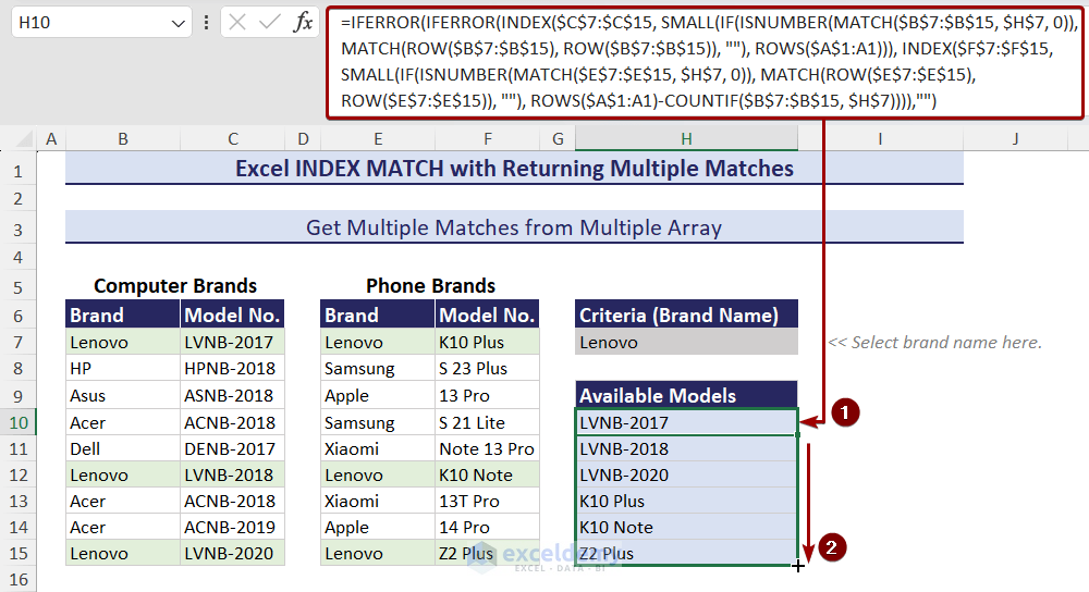
• Look at the GIF below. When we change the brand name from the drop-down list of cell H7, results in the range H10:H15 changes accordingly.

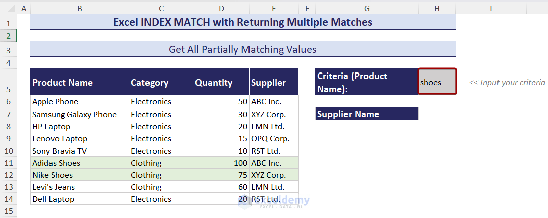
Method 4 – INDEX MATCH Formula to Get All Partially Matching Values

Say, your dataset contains ‘Adidas Shoes’ and ‘Nike Shoes’ and you want to get all corresponding matches where only the ‘shoes’ part matches.

Follow the steps below:

• Set “shoes” as the lookup value in cell H5.

• Insert the following formula in cell H8 and drag the Fill Handle icon:

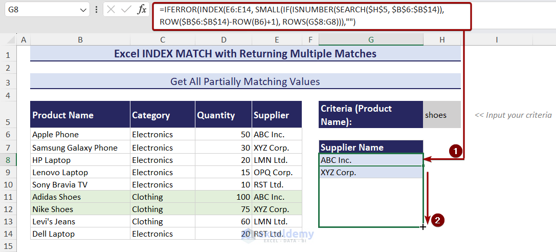
Note:

This formula is not case-sensitive. So, you don’t have to care about the case when setting up the criteria.

Download Practice Workbook

<< Go Back to INDEX MATCH | Formula List | Learn Excel