For illustration, we have a Customer-wise Sales report of a company.
Using this table, we will find the Total Purchase of any Customer across several months using INDEX-MATCH.
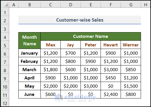
Method 1 – Using SUM Function
Steps:
- Select cell D14 and enter the following formula.
- At the very beginning, go to cell D14 and enter the following formula.
=SUM(INDEX(C6:G11,,MATCH(D13,C5:G5,0)))
We have inserted the range of numbers inside the INDEX function as the array. We have inserted two commas (,). The row and column numbers are entered inside the INDEX function. We have left the placeholder for the row number. This is done so that all the rows will be taken into account. The MATCH function returns the column number. Within the MATCH function, we have inserted the search key as our lookup_value and a lookup_array where we may find the search key. 0 denotes the Exact Match.
- Press ENTER.
The total amount spent by customer Jay will be displayed.
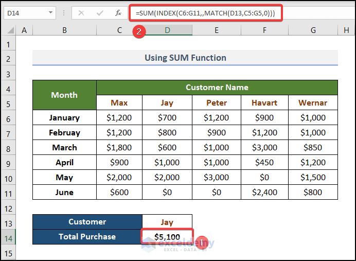
Instead of the SUM function, you can use the SUMPRODUCT function.
- Select cell D14 and insert the following formula.
=SUMPRODUCT(INDEX(C6:G11,,MATCH(D13,C5:G5,0)))
- Press ENTER.
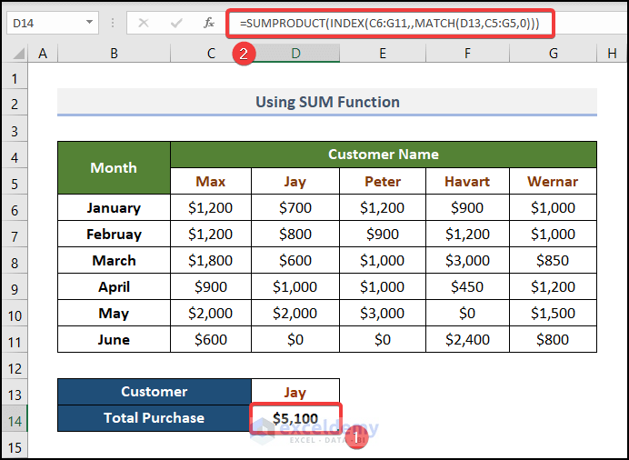
The SUMPRODUCT function works better for an array.
Method 2 – Utilizing AGGREGATE Function
Steps:
- Select cell D14 and enter the following formula.
To do this in our worksheet,
- At first, select cell D14 and write down the following formula.
=AGGREGATE(9,0,INDEX(C6:G11,,MATCH(D13,C5:G5,0)))
To get the sum, we need to use 9 as the function_number. We have used 0 as our behavior_option. The function of the INDEX-MATCH is similar to the previous, it returns the range where we need to execute our operation.
- Press ENTER.
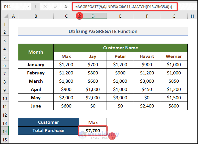
It will show the Total Purchase amount for customer Jay.
Let’s change the criteria (Customer name) and see if the formula works.
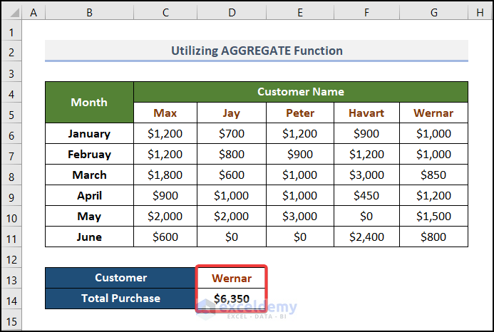
The formula gave us the Total Purchase amount made by Wernar from January to June.
Method 3 – Applying SUBTOTAL Function
Similar to the AGGREGATE function, SUBTOTAL also returns the SUM, AVERAGE, COUNT and MAX.
Steps:
- Select cell D14 and enter the following formula.
- Firstly, go to cell D14 and paste the formula below.
=SUBTOTAL(9,INDEX(C6:G11,,MATCH(D13,C5:G5,0)))
We have chosen 9 since we want to include the hidden values (though we didn’t have any hidden ones).
- Press ENTER.
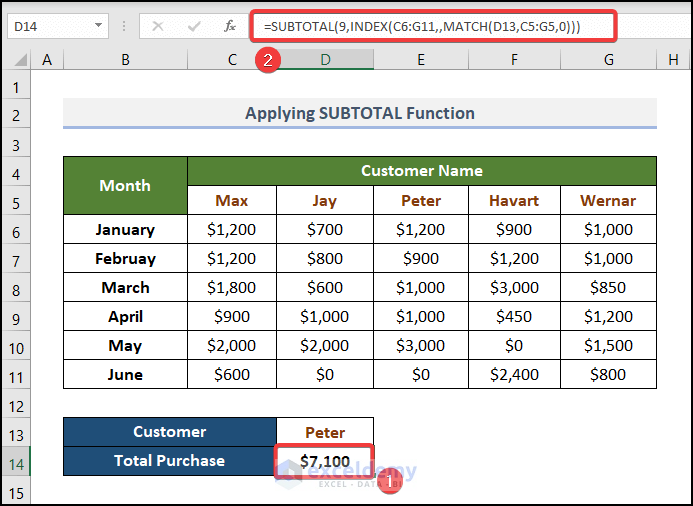
- Let’s check it for Havart.

How to Sum Across Multiple Sheets with INDEX-MATCH Formula
Steps:
We have the Sales amount of 3 different products in 3 different worksheets.
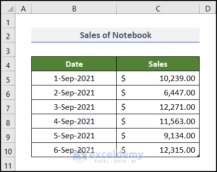
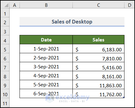
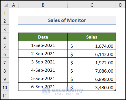
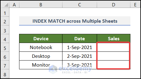
In the following sheet, the Sales of a particular Device or component on a particular Date will be extracted from other corresponding worksheets.
- In the Notebook worksheet, select the entire table (B4:C10).
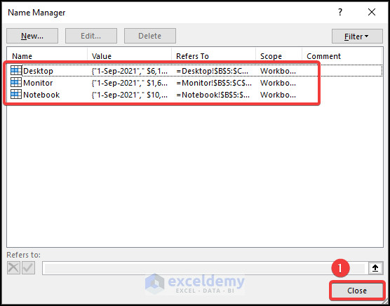
- Go to the Formulas tab and select the Name Manager command on the Defined Names
- Select the New button in the Name Manager dialog box.
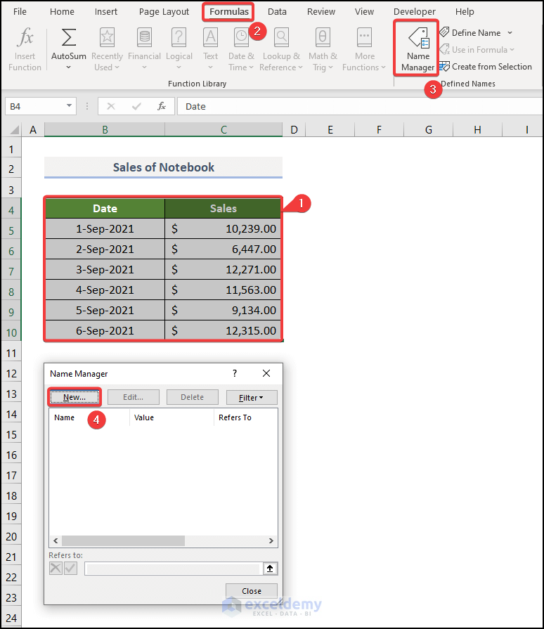
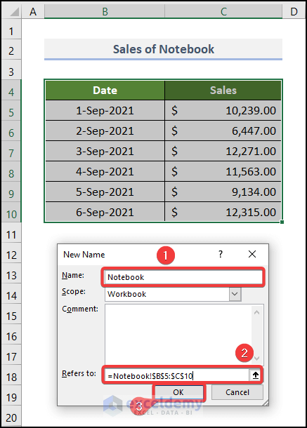
- In the New Name dialog box, enter Notebook in the Name box.
- Give the cell reference of B5:C10 in the Refers to box.
- Click OK.
- Follow the previous step for all other worksheets and name the corresponding tables with the device or components present in the Summary sheet.
- Close the Name Manager dialog box.
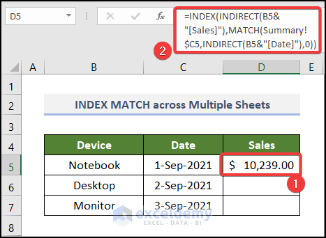
- In the first output cell D5, enter the following formula:
=INDEX(INDIRECT(B5&"[Sales]"),MATCH(Summary!$C5,INDIRECT(B5&"[Date]"),0))
- Press ENTER.
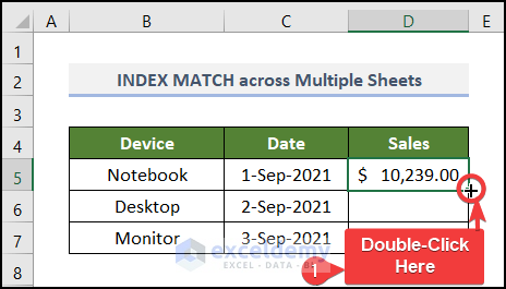
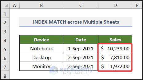
- Use the Fill Handle tool for the remaining cells.
You’ll be able to display the sales of other components or devices on the specified dates.
How to Apply SUMIFS with INDEX MATCH for Multiple Columns
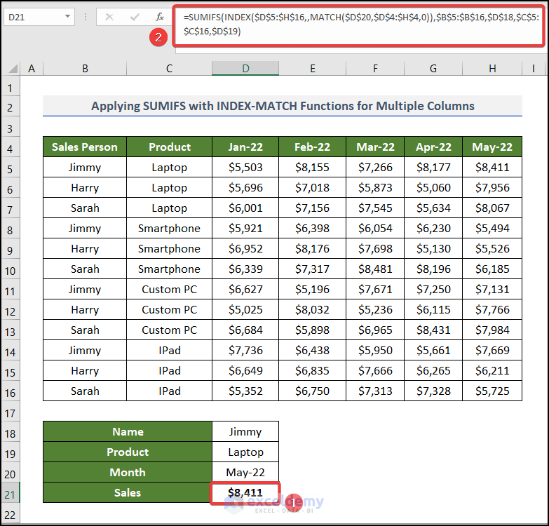
We have the “Monthly Sales of ABC Company” for various Products of 3 Sales Persons.
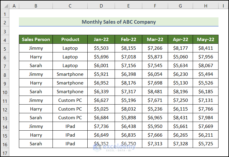
The aim is to find the Sales of a particular Sales Person based on the Month and Product.
Steps:
- Enter the Name of “Sales Person”, Product and Month in cells D18, D19, and D20
- Go to cell D21 and enter the following formula.
=SUMIFS(INDEX($D$5:$H$16,,MATCH($D$20,$D$4:$H$4,0)),$B$5:$B$16,$D$18,$C$5:$C$16,$D$19)
- Press ENTER.
<< Go Back to INDEX MATCH | Formula List | Learn Excel
Get FREE Advanced Excel Exercises with Solutions!

Excellent post, it help me to find a solution for my problem.
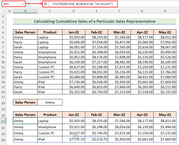
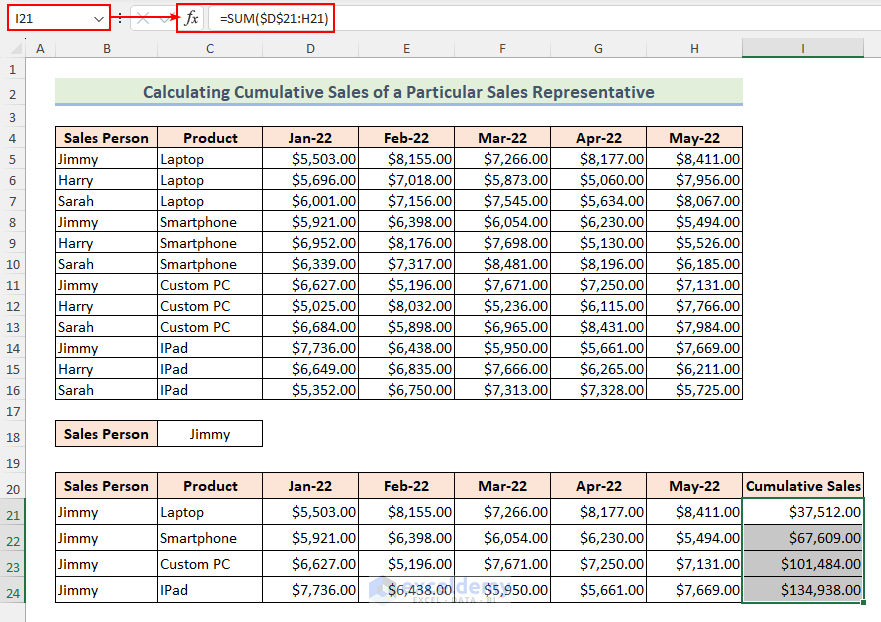
In the last part of the post, I would be interested if there is a way to calculate the cumulative sales let’s say for Jimmy from Jan-22 to May-22.
Thanks so much,
Javier
Hello JAVIER!
Thank you for sharing your problem with us. We have got a very simple solution to your problem. Let’s follow the instructions below to fix your problem.
In cell B21, write down the following FILTER function to filter Jimmy’s data.
=FILTER(B5:H16, B5:B16=C18, "no results")Hence, type the SUM function in cell I21 to calculate cumulative sales.
=SUM($D$21:H21)As a result, you will be able to calculate the cumulative sales of a particular sales representative.
Please download the Excel file for solving your problem and practice with it.
Cumulative Sales.xlsx
If you are still facing issues, please mail us at the address below.
[email protected]
Once again, thank you for your appreciation and for being with us.
Regards
Md. Abdur Rahim Rasel
Exceldemy Team