Here’s an overview of the dataset and an example of the function to extract data by summing based on criteria.

Introduction to SUMIF, INDEX, and MATCH Functions in Excel
The SUMIF Function
- Activity:
Add the cells specified by the given conditions or criteria.
- Formula Syntax:
=SUMIF(range, criteria, [sum_range])
- Arguments:
range- Range of cells where the criteria lies.
criteria- Selected criteria for the range.
sum_range- Range of cells that are considered for summing up.
- Example:
We have a list of PC brands, types of devices, and total sales of these devices across six months.
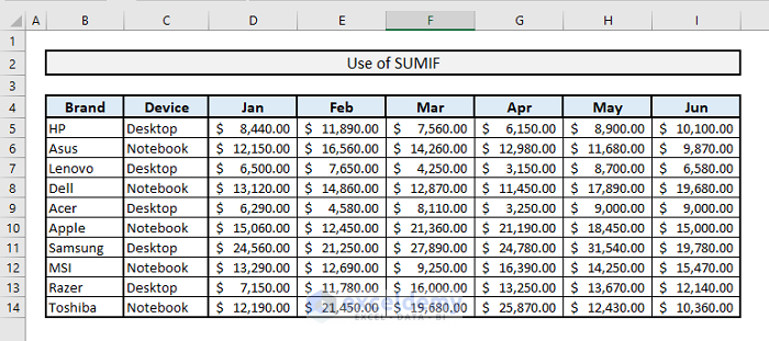
The total sales in the month of May for desktops only of all brands uses the following formula:
=SUMIF(C5:C14,F17,H5:H14)F17 contains the condition Desktop.
The INDEX Function
- Activity:
Returns a value of reference of the cell at the intersection of the particular row & column in a given range.
- Formula Syntax:
=INDEX(array, row_num, [column_num])
OR
=INDEX(reference, row_num, [column_num], [area_num])
- Arguments:
array- Range of cells, columns or rows considered for the values to lookup.
row_num- Row position in the array.
column_position- Column position in the array.
reference- Range of arrays.
area_num- Serial number of array in the reference, if you don’t mention it’ll consider as 1.
- Example:
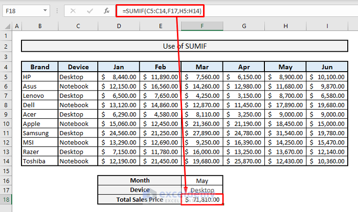
We want to know the value at the intersection of the 3rd row and 4th column from the array of sales prices from the table. We’ll use this formula:
=INDEX(D5:I14,3,4)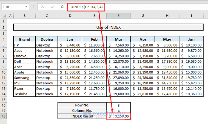
The MATCH Function
- Activity:
Returns the relative position of an item in an array that matches a specified value in a specified order.
- Formula Syntax:
=MATCH(lookup_value, lookup_array, [match_type])
- Arguments:
lookup_value- Cell value that is to be looked for in the range of cells.
lookup_array- Range of cells where lookup value has to be searched for.
match_type- It’s optional. It’ll determine if you want partial or exact match from the array for your lookup value.
- Example:
We’ll get the position of the month June (in F16) from the month headers. In Cell F17, our formula will be:
=MATCH(F16,D4:I4,0)
If we want to know the row position of the brand Dell (F19) from the names of the brands in Column B, the formula in Cell F20 will be:
=MATCH(F19,B5:B14,0)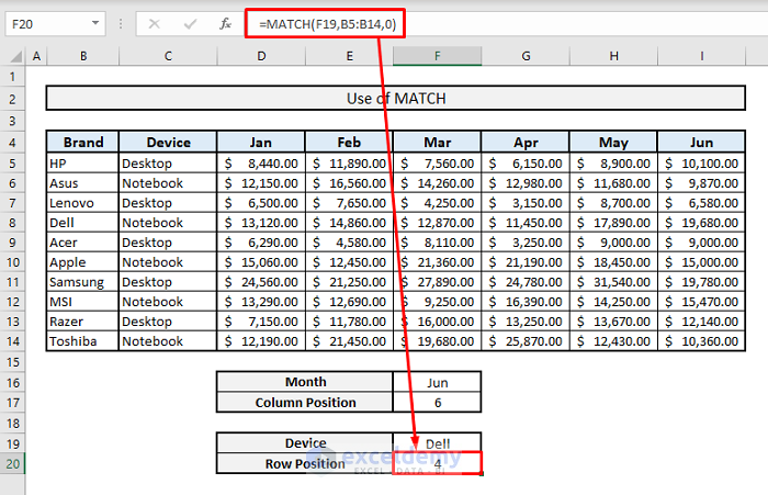
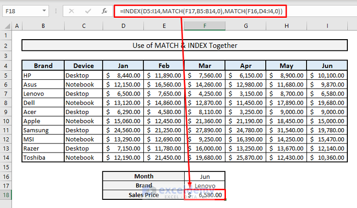
Part 1 – Combining INDEX and MATCH Functions
We want the total selling price of the Lenovo brand in June.
- We listed the month and device type in cells F16 and F17, respectively.
- In Cell F18, insert:
=INDEX(D5:I14,MATCH(F17,B5:B14,0),MATCH(F16,D4:I4,0))- Hit Enter.
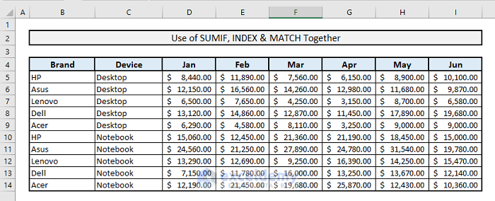
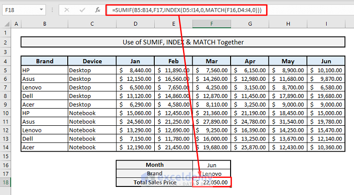
Part 2 – Using SUMIF with INDEX and MATCH Functions in Excel
We’ve modified the dataset to allow duplicated values for brand-device combinations. We’ll find the total sales of Lenovo devices in the month of June.
Steps:
- In the output Cell F18, insert the following formula:
=SUMIF(B5:B14,F17,INDEX(D5:I14,0,MATCH(F16,D4:I4,0)))- Hit Enter.
To find the total sales for desktops, the Sum Range will be C5:C14 and Sum Criteria will be Desktop now. Here’s the formula:
=SUMIF(C5:C14,F17,INDEX(D5:I14,0,MATCH(F16,D4:I4,0)))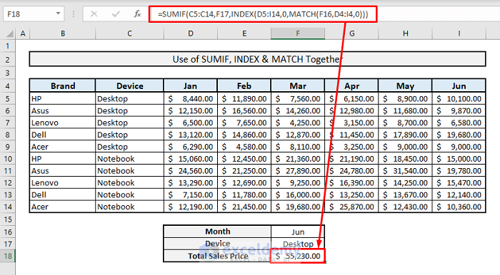
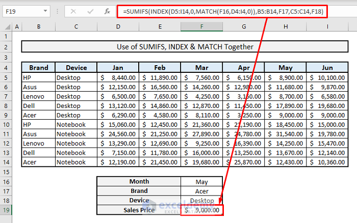
Alternative – Using SUMIFS with INDEX and MATCH Functions in Excel
We’ll find the sales of Acer desktops in the month of May. We’re adding two different criteria from Columns B and C.
Steps:
- Insert the following formula in the result cell F19.
=SUMIFS(INDEX(D5:I14,0,MATCH(F16,D4:I4,0)),B5:B14,F17,C5:C14,F18)- Hit Enter.
Download the Practice Workbook
<< Go Back to INDEX MATCH | Formula List | Learn Excel
Get FREE Advanced Excel Exercises with Solutions!

SUMIFS Columns Multiple with INDEX and MATCH Functions in Excel
Thank you for this.
In your first example in “Use of SUMIF with INDEX & MATCH Functions in Excel” section; how about if I want to find out the total sales for June YTD? So summing all of the months?
Hello Edward, to find out the total sales for one month, you can follow Criteria 7 of the following article.
https://www.exceldemy.com/sum-index-match-multiple-criteria-in-excel/
Here, the Criteria 7 shows how to determine the output based on all Rows & 1 Column with SUM, INDEX, and MATCH functions together. Let us know the result in the reply. Thank you!
Find Total number of Sheets for “.040 ALUM KYNAR”
” “.032 ALUM KYNAR” etc. Thank You
A B
MATERIALS SHEETS
0 0
0 0
0 0
.040 ALUM KYNAR 9
0 0
0 0
.040 ALUM KYNAR 14
0 0
.032 ALUM KYNAR 20
0 0
– –
0 0
0 0
– –
.032 ALUM KYNAR 6
0 0
0 0
.040 ALUM KYNAR 5
.050 ALUM MILL 3
0 0
.050 ALUM KYNAR 9
Hello GARY SHERMAN
Thanks for reaching out and sharing your problem. You want to find the total number of sheets for each material type. To do so, you can use the SUMIF function to reach your goal.
Follow these steps:
As a result, you will see an output like the following image.
Hopefully, the idea will help; Good luck.
Regards
Lutfor Rahman Shimanto
ExcelDemy