Introduction to the XLOOKUP Function
The XLOOKUP function finds a specific value within a range of cells or an array. It then returns the corresponding first match. When there is no exact match, it shows the closest or approximate match.
Syntax:
=XLOOKUP(lookup_value,lookup_array,return_array,[if_not_found],[match_mode],[search_mode])
Arguments:
- Lookup_value: It is the value that we are searching for in a specific column of the range.
- Lookup_array: This is the array in which we are searching for the lookup_value. It can be both row and column.
- Return_array: It is the column from which the corresponding value of the lookup_value will be returned.
Optional Arguments:
- If_not_found: The value will be returned if the lookup_array doesn’t have the lookup_value.
- Match_mode: It is a number denoting the type of match of the lookup_value you want. This is an optional argument. It can contain four values.
- When it is 0, XLOOKUP will search for an exact match (Default).
- When it is 1, XLOOKUP will first search for an exact match. If an exact match is not found, it will match the next smaller value.
- When it is -1, XLOOKUP will first search for an exact match. If an exact match is not found, it will match the next larger value.
- When it is 2, XLOOKUP will first search for an approximate match using Wildcards (Applicable for string lookup values only).
- Search_mode: It is a number denoting the type of search operation conducted on the lookup_array. This is also optional. It can also have four values:
- If it is 1, XLOOKUP will search from top to bottom in the lookup_array (Default).
- When it is -1, XLOOKUP will search from bottom to top in the
- If it is 2, XLOOKUP will conduct a binary search in ascending order.
- When it is -2, XLOOKUP will conduct a binary search in descending order.
Introduction to INDEX-MATCH Functions
The combination of the INDEX and MATCH functions fetches a value from a given location and matches it with the source range.
Syntax:
=INDEX(array,MATCH(lookup_value,lookup_array,match_type),no_of_column)
Arguments:
For the INDEX Function:
- Array: It is a range of cells from which we want to extract a value.
- MATCH(lookup_value,lookup_array,match_type): The row number of the range where the lookup_value matches a specific value in the lookup_array.
- No_of_column: It is the number of the column of the array from which we want to return a value corresponding to the lookup_value.
For the MATCH function:
- Lookup_value: It is the value that we are searching for.
- Lookup_array: It is the array in which we are searching for the lookup_value. It can be both a row and a column.
- Match_type: It is an integer denoting the match we are looking for. This is optional.
- When it is -1, MATCH will first look for an exact match. If an exact match is not found, it will look for the next larger value (Default) (opposite to XLOOKUP).
However, the lookup_array must be sorted in ascending order. Otherwise, it will show an error.
- When it is 1, MATCH will look for an exact match first. In case an exact match is not found, it will look for the next smaller value (opposite to XLOOKUP).
But the condition is that the lookup_array must be sorted in descending order this time. Otherwise, it will show an error.
- When it is 0, MATCH will search for an exact match.
XLOOKUP vs INDEX-MATCH in Excel: 7 Comparisons
Now we have broken down the formula, let’s discuss some similarities and dissimilarities between the two functions. Before going to the main discussions, I will show the major points in a table for your convenience.
| Point of Discussion | Similarity/Dissimilarity | Explanation |
| Column lookup_array | Similarity | Both support a column as the lookup_array. |
| Row lookup_array | Similarity | Both support a row as the lookup_array. |
| No Matching of lookup_value | Dissimilarity | XLOOKUP has the default setup option for not matching the lookup_value. But the INDEX-MATCH does not have. |
| Approximate match | Partial Similarity | XLOOKUP can find the next smaller or larger value when there is no exact match. INDEX-MATCH can also do so, but the lookup_array needs to be sorted in ascending or descending order. |
| Matching Wildcards | Similarity | Both support matching Wildcards. |
| Multiple Values Matching | Partial Similarity | XLOOKUP can find the first or the last value when multiple values match. But INDEX-MATCH can only return the first value that matches. |
| Array Formula | Similarity | Both support the array formula. |
Comparison 1 – XLOOKUP and INDEX-MATCH to Lookup Value in Column
Steps:
- For XLOOKUP, apply the following formula in cell G5:
=XLOOKUP(F5,C5:C16,D5:D16,"Not Found",0,1)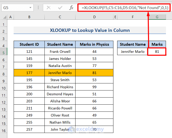
- For INDEX-MATCH, enter the following formula in cell G5:
=INDEX(B5:D16,MATCH(F5,C5:C16,0),3)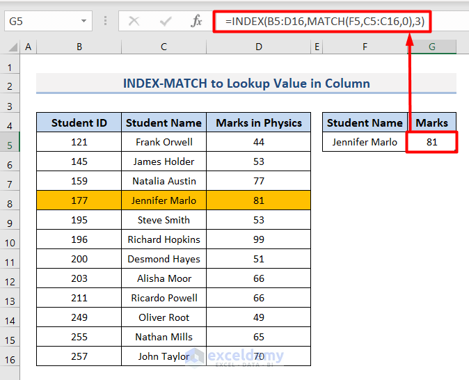
Comparison 2 – XLOOKUP and INDEX-MATCH to Lookup Value in Row
Steps:
- To find out the grade of the 3rd student, enter the XLOOKUP formula in cell G5:
=XLOOKUP("Grade",B4:E4,B7:E7,"Not Found",0,1)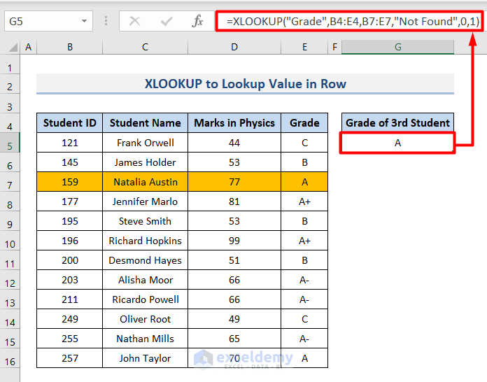
- The INDEX-MATCH formula will be:
=INDEX(B5:E16,3,MATCH("Grade",B4:E4,0))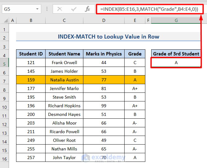
Comparison 3 – XLOOKUP and INDEX-MATCH When No Match Being Found
Steps:
- Enter the following XLOOKUP formula in cell G5:
=XLOOKUP(100,B5:B16,C5:C16,"Not Found",0,1)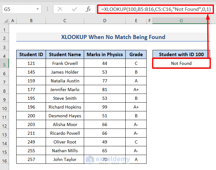
- Enter this INDEX-MATCH formula:
=INDEX(B5:E16,MATCH(100,B5:B16,0),2)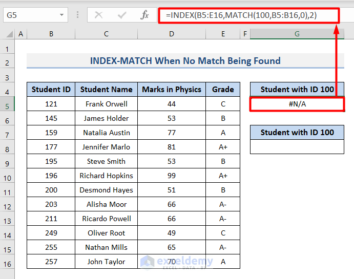
- As it returns an error, you have to use an IFERROR function outside to handle this error.
=IFERROR(INDEX(B5:E16,MATCH(100,B5:B16,0),2),"Not Found")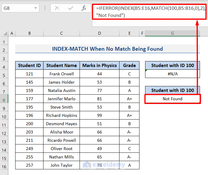
Comparison 4 – XLOOKUP and INDEX-MATCH in Case of Approximate Matches
Steps:
- To find the value, apply this XLOOKUP formula:
=XLOOKUP(50,D5:D16,C5:C16,"Not Found",1,1)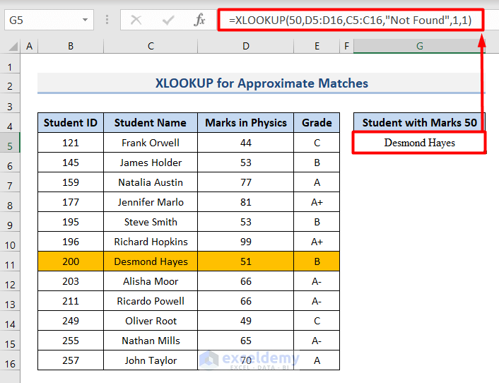
- As you can see, there is no student with a mark of 50. That’s why it is showing the one immediately after 50, 51 by Desmond Hayes.
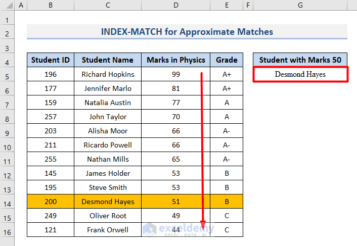
There is the same option in the INDEX-MATCH formula. However, the shortcoming is that you must sort the lookup_array in descending order if you want the next larger value. Otherwise, it will return an error. You have to sort in ascending order to get the next smaller value.
- Insert this formula in cell G5:
=INDEX(B5:E16,MATCH(50,D5:D16,-1),2)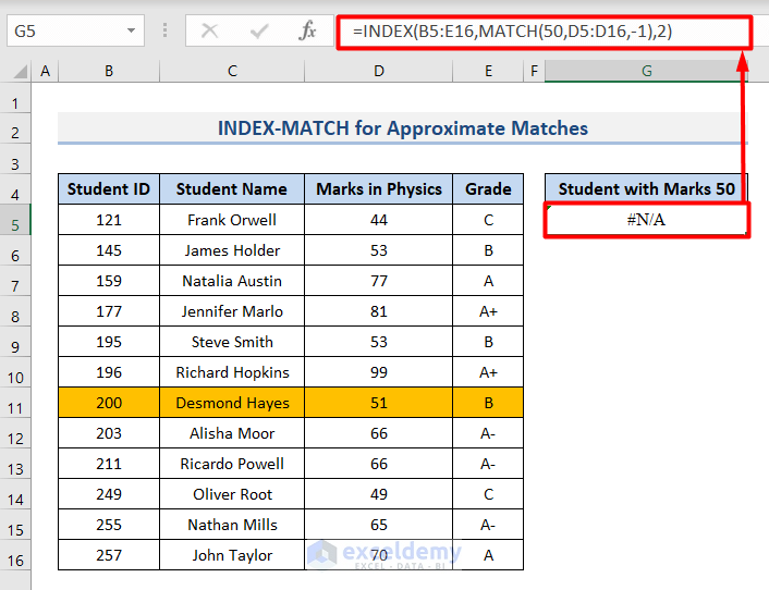
- As a result, you will see an #N/A error.
- Sort the cell range D5:D16 in ascending order, and you will get the correct value.
Comparison 5 – XLOOKUP and INDEX-MATCH in Case of Matching Wildcards
Steps:
- Apply this XLOOKUP formula in cell G5 to get the output.
=XLOOKUP("*Marlo*",C5:C16,C5:C16,"Not Found",2,1)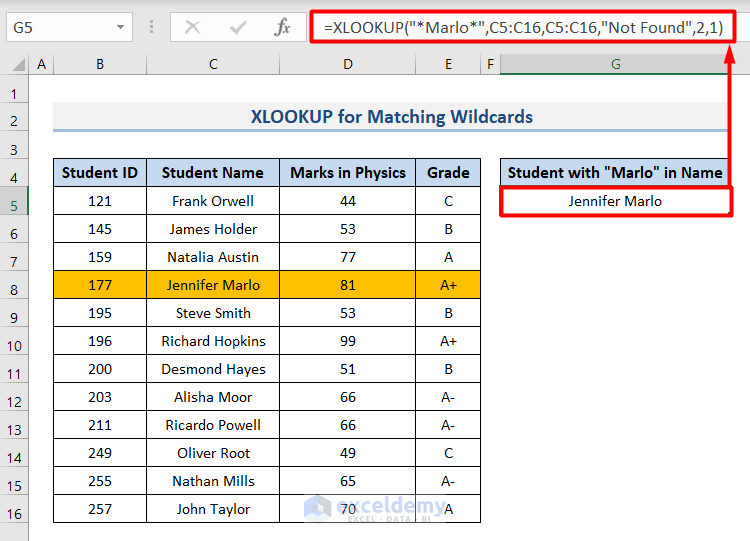
- The INDEX-MATCH formula to accomplish the same task will be like this.
=INDEX(B5:E16,MATCH("*Marlo*",C5:C16,0),2)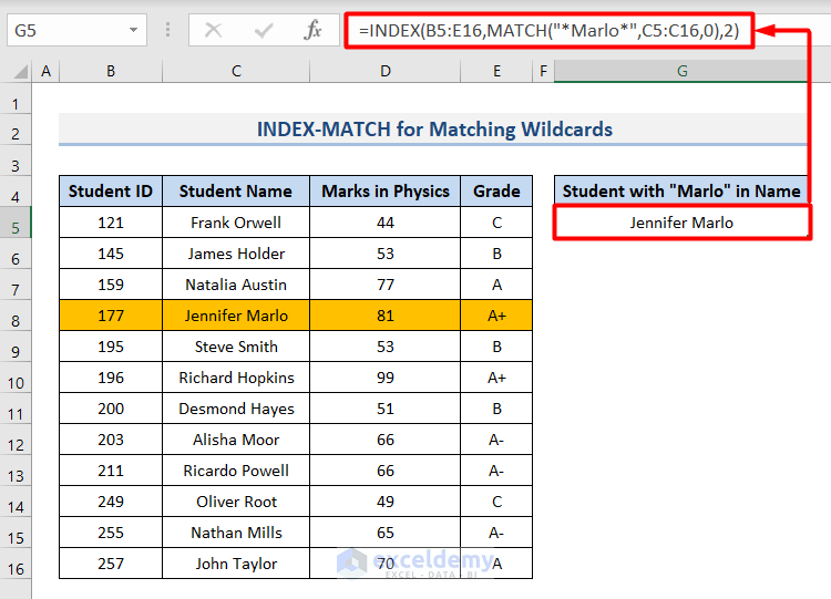
Comparison 6 – XLOOKUP and INDEX-MATCH When Multiple Values Match Lookup Value
Steps:
- To get the first student who got 100, use this XLOOKUP formula in cell G5:
=XLOOKUP(100,D5:D16,C5:C16,"Not Found",0,1)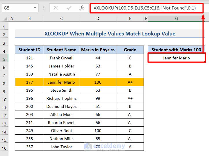
- You will get the last student with 100 using this XLOOKUP formula.
=XLOOKUP(100,D5:D16,C5:C16,"Not Found",0,-1)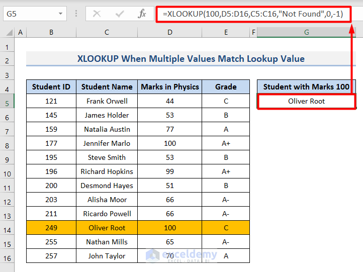
- You will get only the first value that matches with this INDEX-MATCH formula.
=INDEX(B5:E16,MATCH(100,D5:D16,0),2)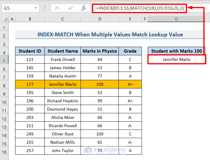
Comparison 7 – XLOOKUP and INDEX-MATCH in Case of Multiple Lookup Values
Steps:
- For the XLOOKUP function, use the following formula:
=XLOOKUP(G5:G8,B5:B16,E5:E16,"Not Found",0,1)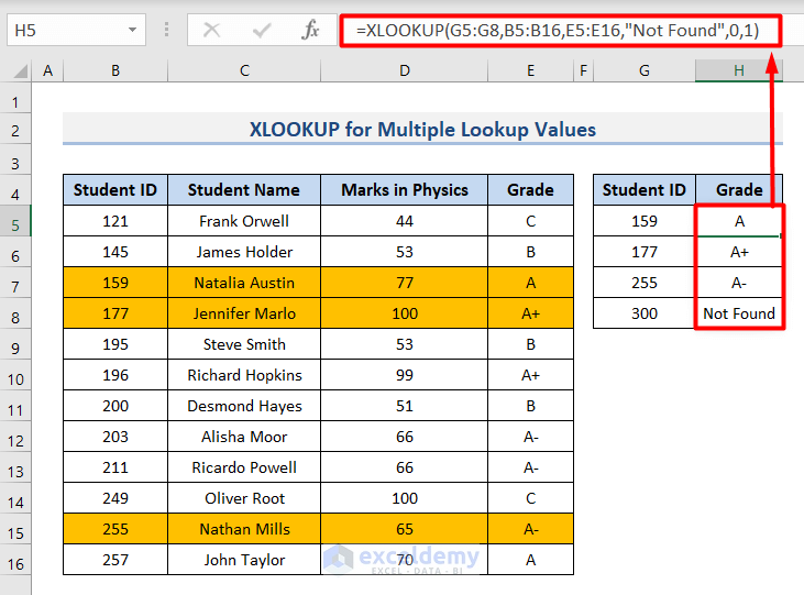
- For INDEX-MATCH, use the following function:
=INDEX(B5:E16,MATCH(G5:G8,B5:B16,0),4)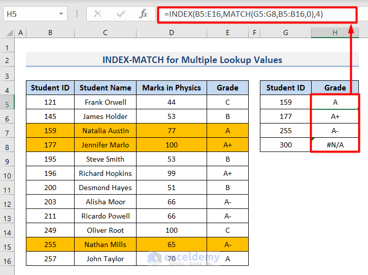
Advantages & Disadvantages of XLOOKUP Function
There are certain advantages and disadvantages of using the XLOOKUP function. Let’s see them in brief.
Advantages
- Set up a default value for cases that do not match.
- Can search for approximate matches without sorting the lookup_array.
- You can search from both the first and last cells of the lookup_array.
Disadvantages
- Works slower than the INDEX-MATCH function.
- Available in Microsoft 365 and 2021 only.
Advantages & Disadvantages of INDEX-MATCH Functions
The INDEX-MATCH functions also have some of the following pros and cons.
Advantages
- Works faster than the XLOOKUP function.
- Available in the old Excel versions.
Disadvantages
- Can’t handle errors when no match is found.
- The lookup_array needs to be sorted for approximate matches.
- Returns only the first value when multiple values match the lookup_value.
Download the Practice Workbook
Download the workbook to practice.
<< Go Back to INDEX MATCH | Formula List | Learn Excel
Get FREE Advanced Excel Exercises with Solutions!

RIP Index-Match. Having begun to use XLOOKUP, I don’t see where INDEX-MATCH is to be preferred. XLOOKUP is much easier to us. The only wonder is why it took Microsoft so long to update their archaic formulas.
Hi,
I’m struggling to find the right formula to multiply units by rates.
I have different materials with different units and rates are depend on quantities.
I have a more than 2000 row spreadsheet and units also varies that means that the formula also need to find the unit on sheet 1. Rate criteria can also change on sheet 1.
Many thanks for your help!
Details on Sheet 1
Unit Rate1(not exceeding) Rate2(not exceeding) Rate3(not exceeding) Rate4(exceeding)
day
h
m (QB) 10 50 200 200
m
m2 (QB) 10 50 150 200
m2
Details on Sheet 2
Description Unit Quantity Rate 1 Rate 2 Rate 3 Rate 4 Price
path m (QB) 9 11 13 13.5 14
road m (QB) 51 5 10 15 20
wall m2 (QB) 35 10 15 20 25
wood m 20 11
paint m2 150 12
And I’m looking for the price.
Many thanks for your help!
Niki
Hi Niki,
To find out the price, you need to calculate the product of unit and unit quantity. Your sheet 1 denotes the unit of rate 1, rate 2, rate 3, and rate 4. The unit quantity will be found in sheet 2. So, in that case, you can apply the VLOOKUP formula to get the specific unit and unit quantity. You can use the following formula to calculate.
=VLOOKUP(J8,$B$7:$C$12,2,FALSE)*VLOOKUP(J8,Sheet1!$B$4:$C$8,2,FALSE)
=VLOOKUP(J8,$B$7:$C$12,2,FALSE):
First, you need to define the value you are looking for. Here, J8 refers to the lookup value. After that, define the table array where you think the required answer can remain. Then, define the column number of the expected result. Finally, use false to get the exact match. Then, we have to multiply the result of the first VLOOKUP by the result of the second VLOOKUP.
VLOOKUP(J8,Sheet1!$B$4:$C$8,2,FALSE):
As we put the unit in sheet 1, we have to look up the rate 1 unit by utilizing the VLOOKUP function. First, define rate 1 as the lookup value. Then, set the table array in sheet 1. After that, define the column number of the expected result. Finally, use false to get the exact match.
The product of these two values will give the price of rate 1. Do the same procedure for other cases.
Do you get your preferred answer? check on it. Otherwise, give us a more accurate question. We are always ready to help you.
Thank you.