Method 1 – Deleting Blank Cells Manually
Steps:
- Hover the cursor until a downward pointing arrow appears >> left-click to select the column, here it is Column C.
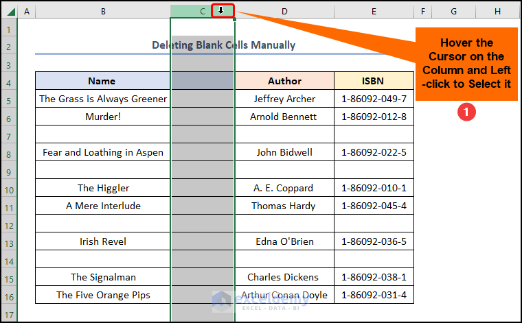
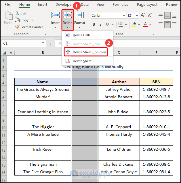
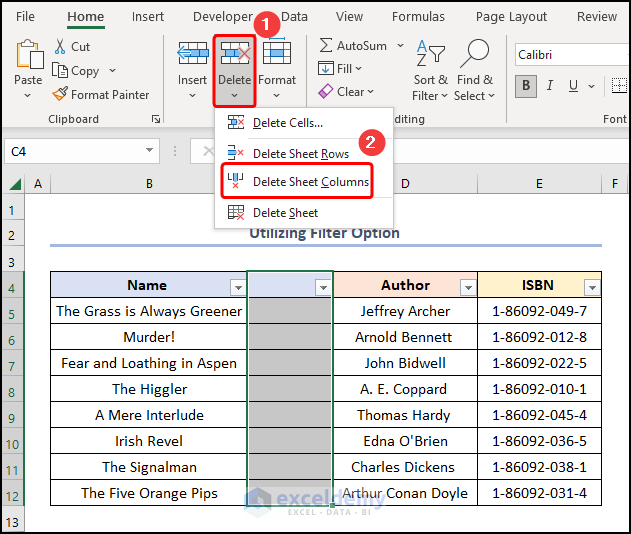
- Click the Delete drop-down >> press Delete Sheet Columns.
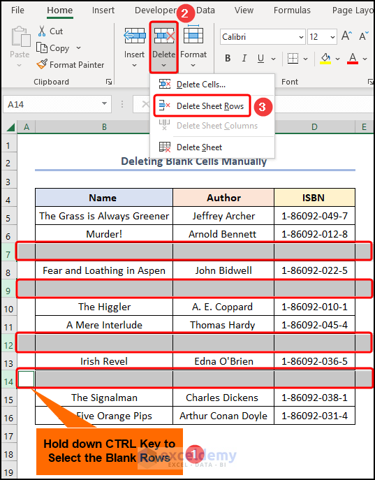
- Hold down the CTRL Key >> left-click on the row numbers to select multiple rows, in this case, rows 7, 9, 12, and 14 >> choose the Delete Sheet Rows option.
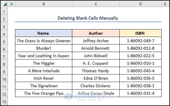
Remove blank cells in Excel and shift data up.
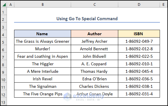
Method 2 – Using Go To Special Command
Steps:
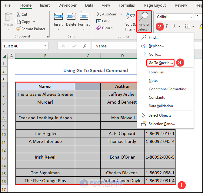
- B4:E16 cells >> click Find & Select drop-down >> select Go To Special.
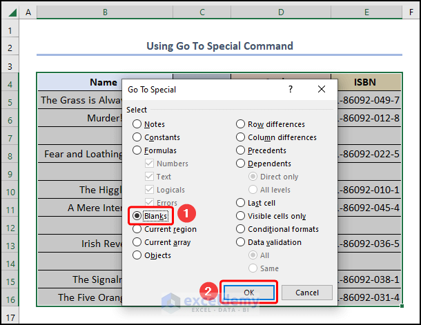
- Go To Special window, click the Blanks button>> hit OK.
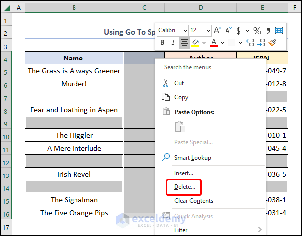
- Right-click to open the Context Menu >> choose Delete.
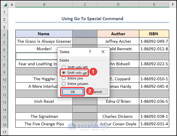
- Check the Shift cells up the option to remove all the blank rows.
- Select the blank column >> select the Shift cells left option >> press OK.

Deletes the blank cells as shown in the image below.
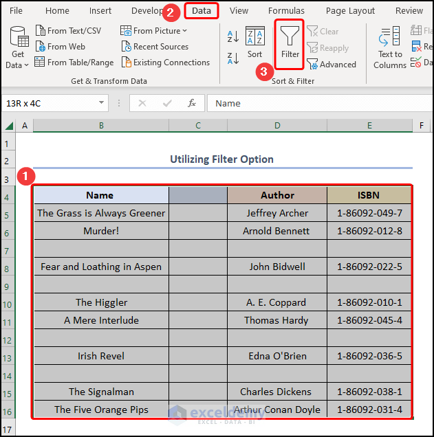
Method 3 – Utilizing Filter Option
Steps:
- Highlight the B4:E16 cells >> move to the Data tab >> click the Filter option.
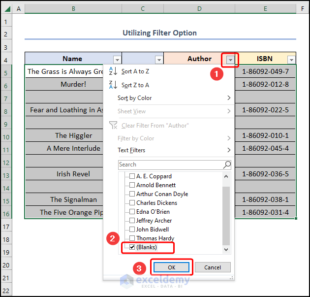
- Click any down-arrow button >> check the Blanks option >> enter the OK button.
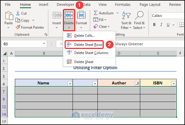
- Delete Sheets Rows to remove all the blank rows.
- Click the down-arrow button >> check the Select All option >> click on OK.
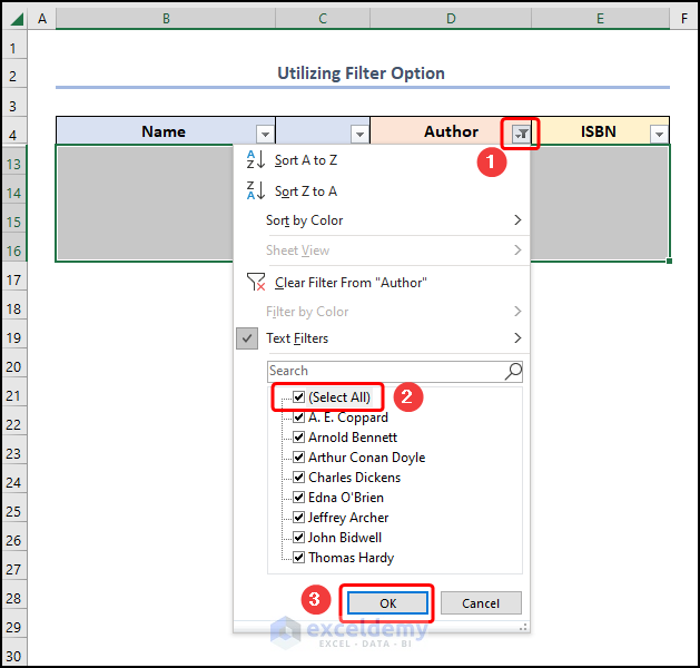
- Select the blank column >> press Delete Sheet Columns.
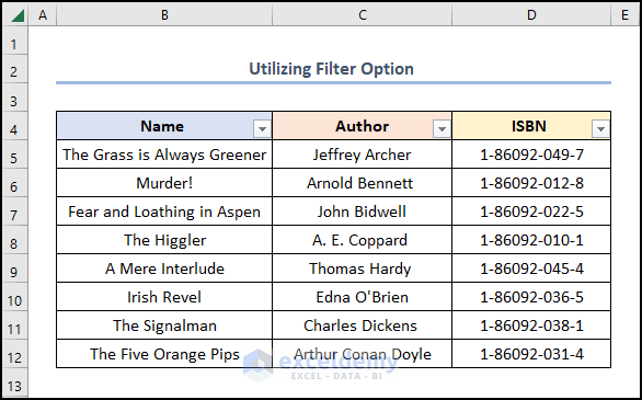
The results should look like the picture shown below.
Method 4 – Applying Sort Feature
Steps:
- Select the B5:E16 cells >> navigate to the Data tab >> click the Sort feature.
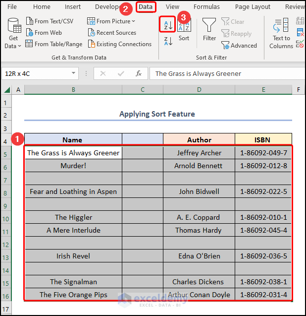
- Select the blank rows >> use the CTRL + – (Minus) keys to delete them.
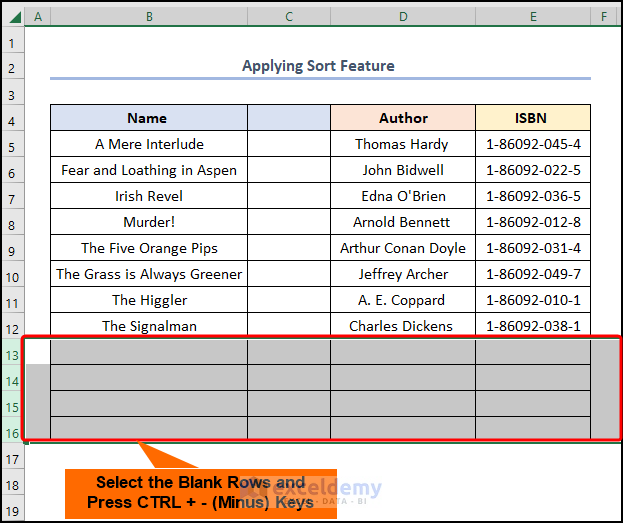
- Select the blank column >> press CTRL + – (Minus) keys to delete the column.
![]()
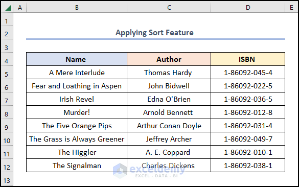
Your results should resemble the screenshot below.
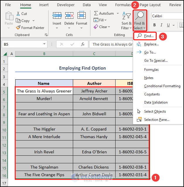
Method 5 – Employing Find Option
Steps:
- Select the B5:E16 cells >> jump to the Find option in the Find & Select drop-down.
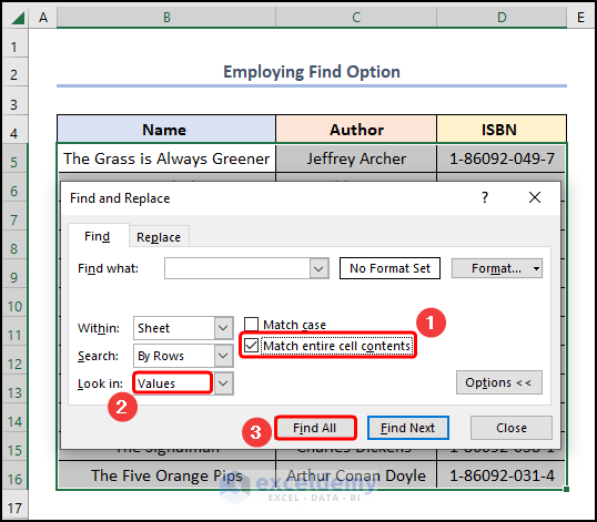
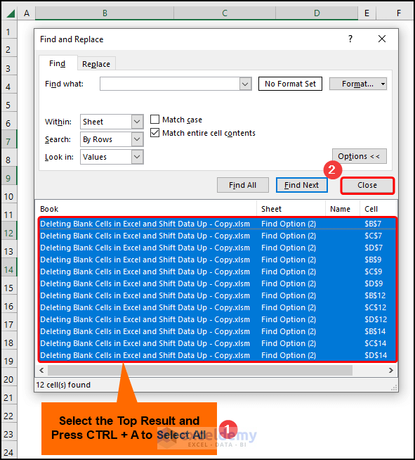
- Find and Replace, check the Match entire cell contents option >> in the Look in field, select Values option >> press Find All.
- The top result and press the CTRL + A keys to select all >> hit Close.
- Apply the Delete Sheet Rows option.
![]()
The results should appear in the screenshot below.

Method 6 – Incorporating Advanced Filter Menu
Steps:
- Follow the steps shown in the animated GIF shown below.
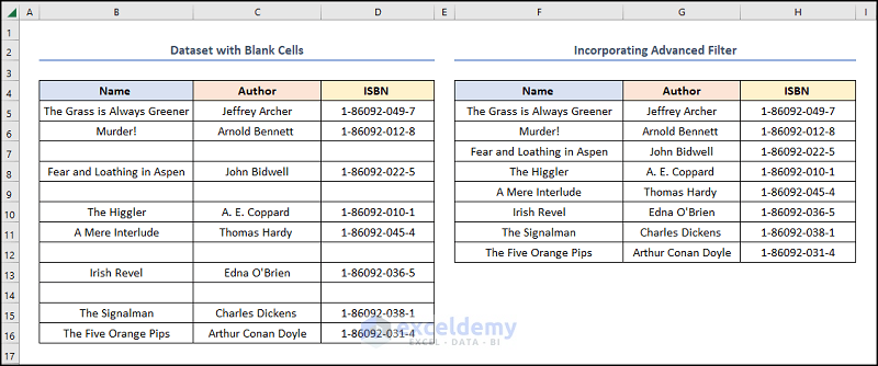
The final output should look like the figure below.
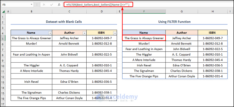
Method 7 – Using FILTER Function
Steps:

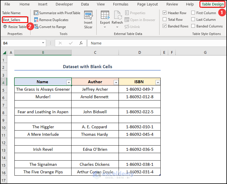
- Proceed to the Table Design tab >> rename the Table as “Best_Sellers”.
- Move to the F5 cell >> insert the formula into the Formula Bar.
=FILTER(Best_Sellers,Best_Sellers[[Name ]]<>"" )
- FILTER(Best_Sellers,Best_Sellers[[Name ]]<>”” ) → filter a range or array. Here, Best_Sellers is the array argument, while Best_Sellers[[Name ]]<>”” is the include argument that removes the blank rows in the given array.
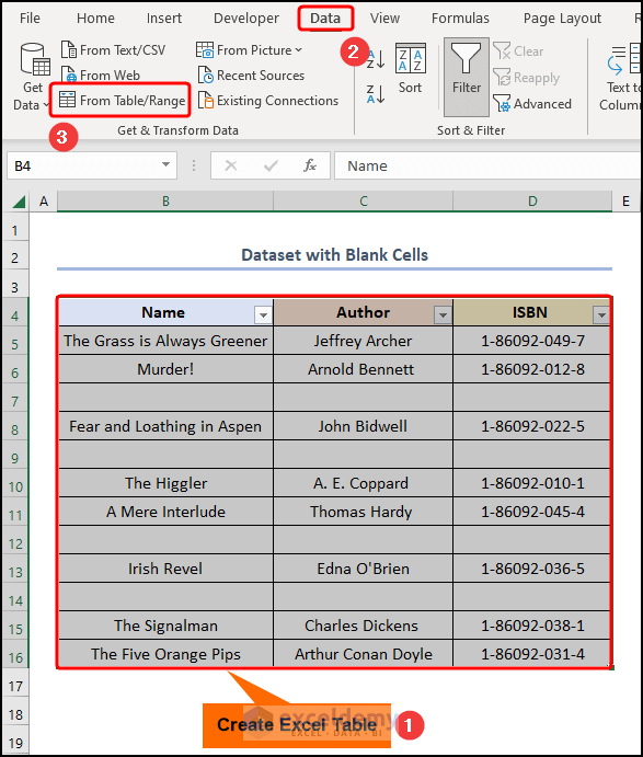
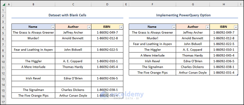
Method 8 – Implementing PowerQuery Option
Steps:
- Insert an Excel Table as shown previously >> go to the Data tab, and click the from Table/Range option.
- Follow the steps in real time as shown in the GIF.
- Move to the Close & Load drop-down >> select the Close & Load To option.
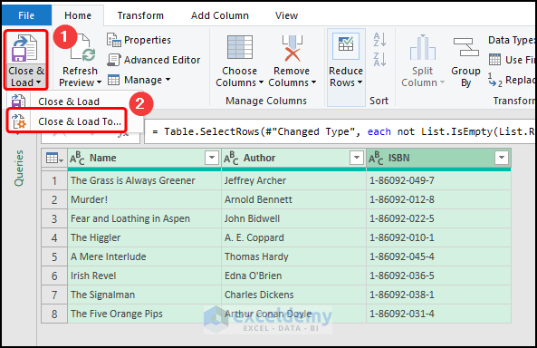
- Choose the Existing worksheet option and select the F4 cell.
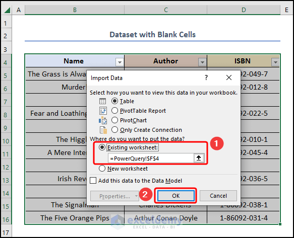
The results should look like the screenshot below.
How to Delete Empty Cells and Shift Data Up Using Excel VBA
Steps:
- Navigate to the Developer tab >> click the Visual Basic button.
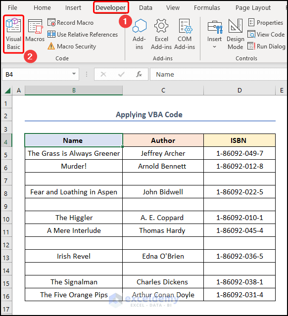
This opens the Visual Basic Editor in a new window.
- Go to the Insert tab >> select Module.
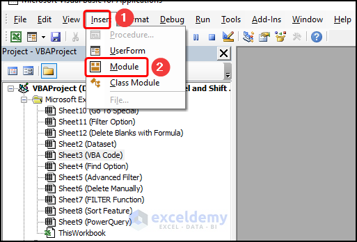
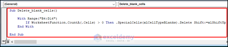
Copy the code from here and paste it into the window below.
Sub Delete_blank_cells()

    With Range("B4:D16")
        If WorksheetFunction.CountA(.Cells) > 0 Then .SpecialCells(xlCellTypeBlanks).Delete Shift:=xlShiftUp
    End With

End Sub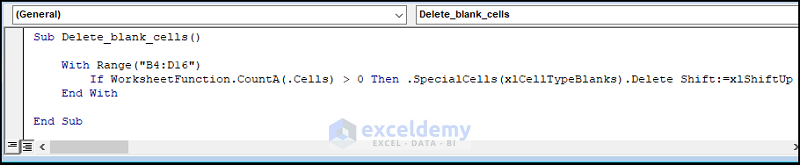
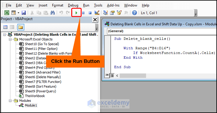
- The sub-routine is given a name, here it is Delete_blank_cells().
- Use the With statement and Range property to set the range of the dataset.
- Use the If statement and CountA function to check whether the cell is blank, in which case, use the Delete method to remove the blank rows.
- Click the Run button or press the F5 key to execute the macro.
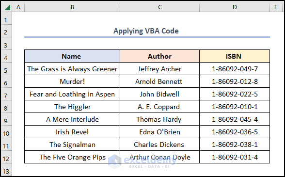
The results should look like the image given below.
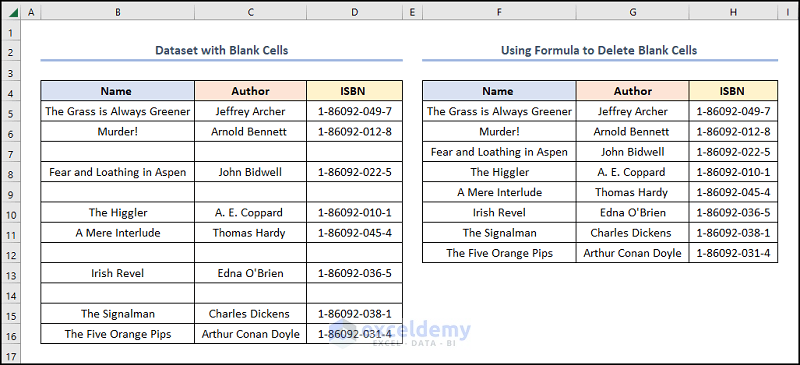
How to Delete Blank Rows in Excel and Shift Data Up Using Formula
Steps:
- Copy and paste the expression into the F5 cell.
=IFERROR(INDEX(B:B,SMALL(IF(B$5:B$16<>"",ROW(B$5:B$16)), ROWS(B$5:B5))), "")
The B5:B16 cells refer to the “Name” column.
- ROW(B$5:B$16)→ returns the serial number of the row.
- Output → {5;6;7;8;9;10;11;12;13;14;15;16}
- ROWS(B$5:B5) → returns the total row numbers in the given range.
- Output → 1
- IF(B$5:B$16<>””,ROW(B$5:B$16)) → checks whether a condition is met and returns one value if TRUE and another value if FALSE. Here, B$5:B$16<>”” is the logical_test argument that checks the B5:B16 range for blanks. The function returns the ROW(B$5:B$16) if the test holds TRUE (value_if_true argument) otherwise it returns FALSE (value_if_false argument).
- Output → {5;6;FALSE;8;FALSE;10;11;FALSE;13;FALSE;15;16}
- SMALL(IF(B$5:B$16<>””,ROW(B$5:B$16)), ROWS(B$5:B5)) → becomes
- SMALL({5;6;FALSE;8;FALSE;10;11;FALSE;13;FALSE;15;16}) → returns the kth smallest value in data set.
- Output → 5
- INDEX(B:B,SMALL(IF(B$5:B$16<>””,ROW(B$5:B$16)), ROWS(B$5:B5))) → becomes
- INDEX(B:B,5) → returns a value at the intersection of a row and column in a given range. In this expression, the B:B is the array argument which is the “Name” column. Next, 5 is the row_num argument that indicates the row location.
- Output → “The Grass is Always Greener”
- IFERROR(INDEX(B:B,SMALL(IF(B$5:B$16<>””,ROW(B$5:B$16)), ROWS(B$5:B5))), “”) → becomes
- IFERROR(“The Grass is Always Greener”, “”) → returns value_if_error if the expression has an error and the value of the expression itself otherwise. Here, “The Grass is Always Greener” is the value argument, and “” is the value_if_error argument.
- Output → “The Grass is Always Greener”
The results should look like the picture shown below.
Download Practice Workbook
Related Articles
- How to Remove Blank Lines in Excel
- How to Ignore Blank Cells in Range in Excel
- How to Leave Cell Blank If There Is No Data in Excel
<< Go Back to Blank Cells | Excel Cells | Learn Excel
Get FREE Advanced Excel Exercises with Solutions!
