A cell is the smallest unit of an Excel worksheet. Each cell has a unique address. The cell address is a combination of a column letter and a row number.
What Is a Cell in Excel?
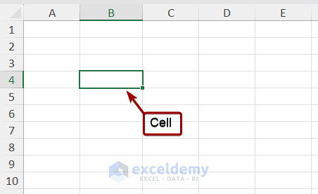
The cell is the smallest unit of the Excel worksheet. It is the intersection point of a row and column and is referred to as the combination of a letter and a number e.g., A1.
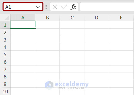
We can see the address of the active cell in the Name Box.
The currently selected cell in the worksheet is called the Active Cell.
How to Select Cells in Excel?
Selecting a Single Cell:
- Click the cell to select it.
Selecting a Range of Contiguous Cells:
- Select a single cell. Left-click and drag the cursor in any direction to select multiple contiguous cells.
Or hold Shift and press the arrow keys on the keyboard to drag the selection cursor over the cells.
Selecting Non-Contiguous Cells:
- To select multiple non-contiguous cells, press and hold Ctrl and select cells one by one.
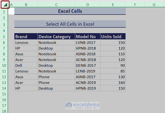
Selecting All Cells:
- Select any cell of a range or table and press Ctrl+A twice.
 or hover your mouse to the place where row and column headers merge and click.
How to Insert and Delete Cells in Excel?
Inserting Cells:
To insert a new blank cell after C6 in the same column:
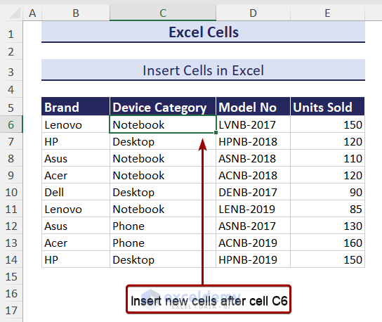
- Place the cursor over C7 and right-click.
- Select Insert in the Context Menu.
- Choose Shift cells down in Insert.
Content in C7:C14 will be moved one cell down, and a new blank cell will be created in C7.
- To insert N cells, select N cells. Right-click and follow the the same procedure described above.
If you choose Shift cells right, the existing cells will be shifted rightwards.
Deleting Cells:
To delete C7:
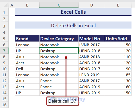
- Select C7. Right-click and choose Delete.
- Choose Shift cells up in Delete.
C7 is deleted, and the other cells in column C are shifted up
How to Resize Excel Cells?
To resize B4:
1. Use the Resize Cursor
- Place the cursor on the right edge of column B.
- Left-click and drag the mouse to the right or left to increase or decrease the width.
- To modify the height, place the cursor on the bottom edge of row 4.
- Left-click and drag the mouse up or downwards to decrease or increase the cell height.
2. Resize a Cell in the Context Menu
- Place the mouse on the heading of column B and right-click.
- In the Context Menu, select Column Width.
- Insert the width and click OK.
- Place the mouse on the heading of row 4.
- Select Row Height in the Context Menu.
- Enter the height and click OK in Row Height.
How to Edit a Cell in Excel?
1. Double-clicking the Left Button of the Mouse
- Select a cell and double-click the left mouse button.
2. Using Keyboard
- Select a cell and press F2.
On a laptop, press Fn, and then F2.
How to Refer to a Cell in an Excel Formula?
You refer to a cell in an Excel formula using a cell reference. A cell reference is the address of a cell.
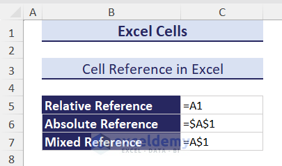
There are 3 types of cell references:
Relative Cell Reference: In relative cell referencing, both the column and row change when you drag or copy the formula to another location. Example: =A1
Absolute Cell Reference: In absolute cell referencing, both the column and row remain unchanged. The absolute sign ($) is used before the column and row number. Example: =$A$1
Mixed Cell Reference: Every components of a cell will change. The absolute sign is used before the column or row number. Example: =A$1. If you copy this cell reference, only the column letter will change its relative position.
How to Copy, Cut, and Paste Cells in Excel?
Copying and Pasting Cells:
- Use Ctrl+C (copy) and Ctrl+V (paste).
Or,
- Select the cell or range (E5:E14) and click Copy in Clipboard.
- Go to F5 and click Paste in Clipboard.
Cut and Paste Cells:
- To cut, press Ctrl+X. Press Ctrl+V to paste.
Or,
- Select E5:E14 and click Cut in Clipboard.
- Go to F5 and select Paste in Clipboard.
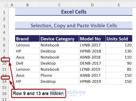
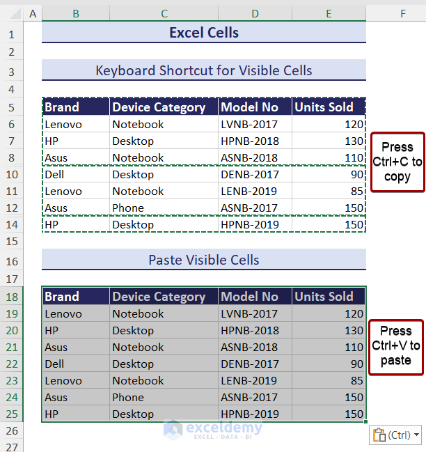
How to Copy Visible Cells Only in Excel?
In the dataset below, rows 9 and 13 are hidden. To copy and paste B5:E14 to another location excluding rows 9 and 13:
1. Applying a Keyboard Shortcut
- Select B5:E14 and press Alt + :. only visible cells are selected.
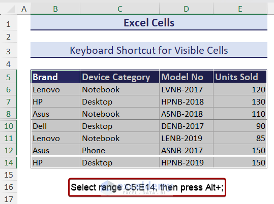
- Press Ctrl+C to copy.
- Go to B18 and press Ctrl+V to paste.
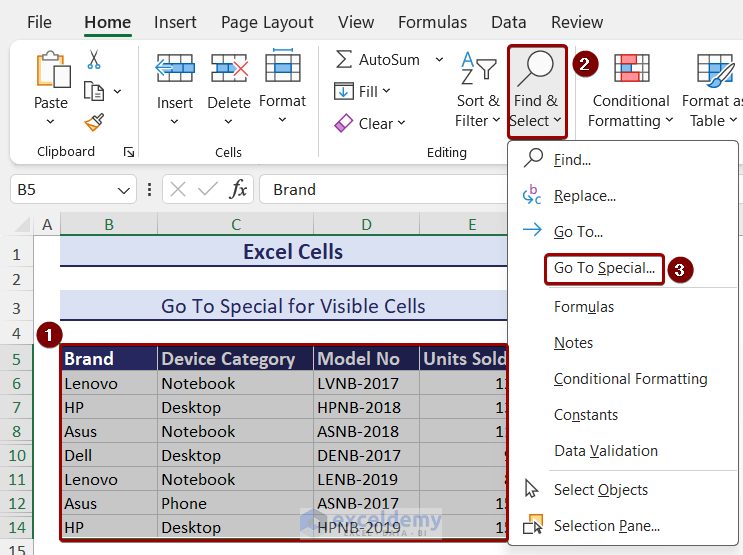
2. Using the Go To Special Feature
- Select B5:E14 > Click Find & Select in Editing > Select Go To Special.
- In Go To Special, click Visible cells only in Select.
- Click OK.
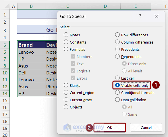
Only visible cells are selected.
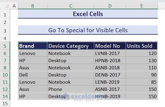
- Copy and paste visible cells only using Ctrl+C and Ctrl+V.
How to Protect Cells in Excel?
Steps:
- Click Select All.
- Press Ctrl+1 to open the Format Cells dialog box.
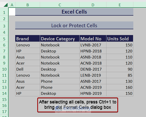
- Select Protection.
- Uncheck Locked and click OK.
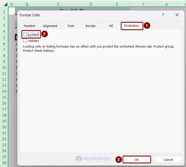
All cells are unlocked. To lock B5:B14 only:
- Select B5:B14.
- Open the Format Cells dialog box.
- Check Lock in Protection.
- Click OK.
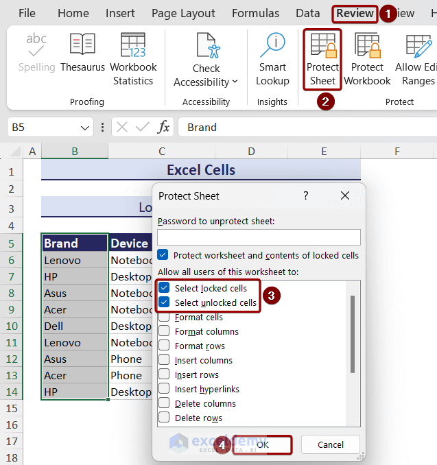
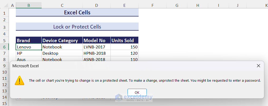
- Go to the Review tab > Click Protect Sheet in Protect.
- Check Select locked cells and Select unlocked cells.
- Click OK.
The warning shown below will be displayed when clicking any protected cell in B5:B14.
- To protect the entire worksheet, lock all cells in Protection. Protect the sheet as shown above.
How to Navigate Between Cells in Excel?
Use arrow keys to navigate in Excel: move up, down, left, and right.
There are other keyboard keys with more features.
| Key | Function |
|---|---|
| Tab | Move rightward |
| Shift + Tab | Move leftward |
| Ctrl + Home | Go to the first cell of the sheet, A1 |
| Page Up | Go to the previous page |
| Page Down | Go to the next page |
How to Move or Shift Cells in Excel?
- Select E5:E14 and move the cursor to the border of the selection area.
- The cursor becomes a move cursor. Press and hold the left button of the mouse.
- Drag the cursor and select a location.
You can also move cells by cutting and pasting.
How to Swap Cells in Excel?
Swap Adjacent Cells:
To swap cells column-wise, here E6 and E7.
- Select E6 and press and hold Shift.
- Move the cursor to the bottom edge of E6.
- Slowly drag the mouse downward to E8. Release Shift and mouse.
E6 and E7 were swapped.
To swap cells row-wise, here C9 and D9.
- Holding Shift and place the mouse at the right border of C9.
- Drag the left-mouse button rightward to E9. Release Shift and mouse.
C9 and D9 were swapped.
Swap Non-Adjacent Cells:
To swap two non-adjacent cells, here E7 and E12:
- Swap E7 to E12.
- E12 will be shifted to E11.
- Swap E11 to E7.
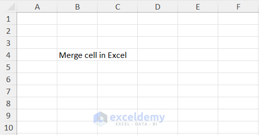
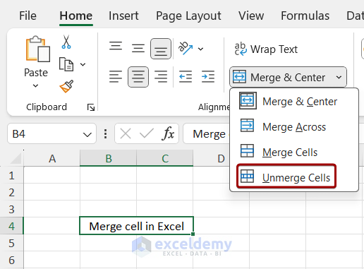
How to Merge and Unmerge Cells in Excel?
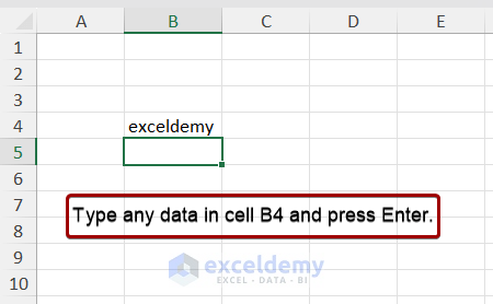
You want to write a sentence in B4 that exceeds its borders.
- Select B4 and C4 and click Merge & Center.
- Choose an option.
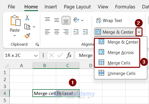
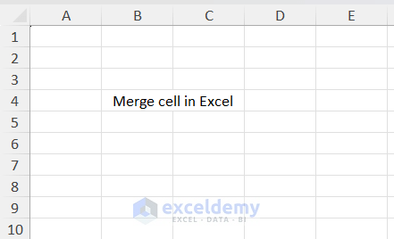
- Cells are merged.
- To unmerge cells, select Unmerge Cells in Merge & Center.
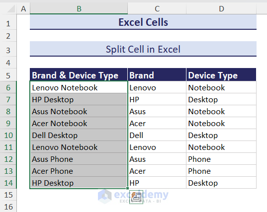
How to Split Data in an Excel Cell?
In column B, the brand and device type are combined. To split the brand and device type into separate columns:
- Select B6:B14.
- Go to the Data tab > Text to Columns in Data Tools.
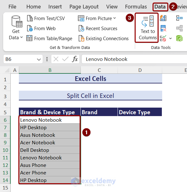
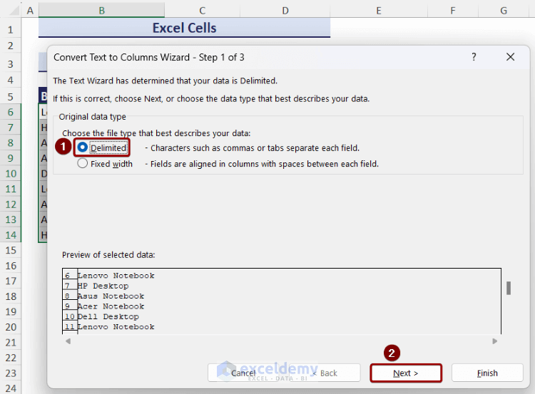
- The Convert Text to Columns Wizard is displayed.
- Check Delimited in Choose the file type that best describes your data:
- Click Next.
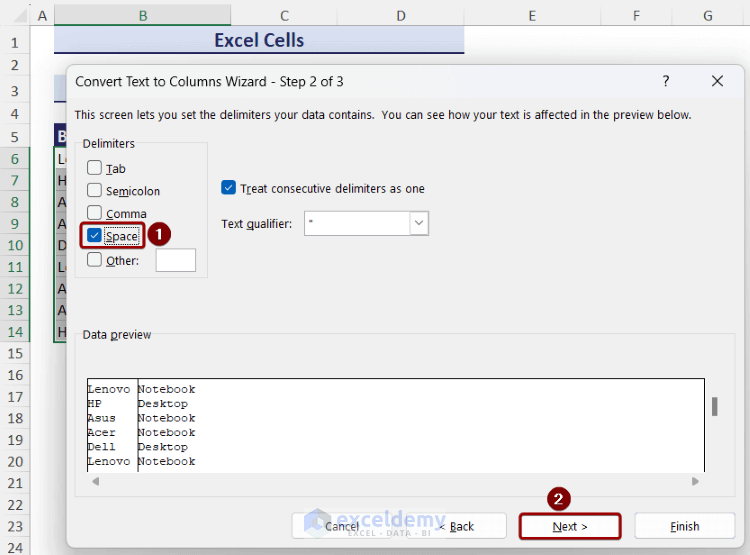
- In Convert Text to Columns Wizard, check Space as Delimiter.
- Click Next.
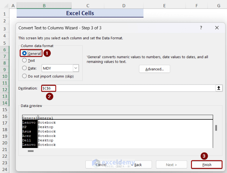
- In Convert Text to Columns Wizard, select General in Column data format.
- In Destination, select C6.
- Click Finish.
Brand name and device type are split into two different columns.
How to Edit Cell Content in Excel?
Insert Content in an Excel Cell:
- Enter content in a selected cell. Press Enter and data will be inserted.
Delete or Clear Cell Content:
- Select B4 > Click Clear > Select Clear Contents.
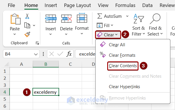
Content is deleted.
You can also select a cell containing data and press Delete.
Excel Cells: Knowledge Hub
<< Go Back to Learn Excel
Get FREE Advanced Excel Exercises with Solutions!
