How to Remove Unused Cells in Excel (10 Methods)

Method 1 – Using the Go To Special Command

Steps:

Select the data range (B4:E12).
Press F5 or Ctrl + G to bring up the Go To dialog box.
Click Special from the dialog box.

In the Go To Special dialog, choose Blanks from the list of options and click OK.

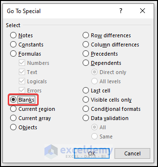
All blank cells in the range will be highlighted.
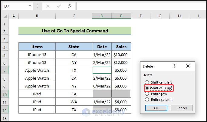
Press Ctrl + – (minus) to open the Delete dialog.
Choose an appropriate delete option (e.g., Shift cells up) based on your data and requirements.
Click OK to delete the blank cells and move non-empty cells up.

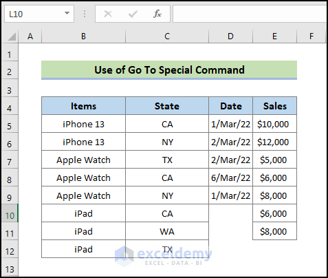
The unused cells have been removed.

Note:

Ensure you select the correct dataset; otherwise, this process may alter the sequence by replacing empty cells with values from other cells.
You can access the Delete dialog by right-clicking on the selection or navigating to Home, select Cells, choose Delete and clicking on Delete Cells.

Method 2 – Applying Filter Option to Remove Rows with Unused Blank Cells

Steps:

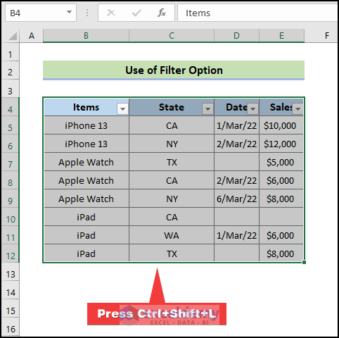
Select the range.
Press Ctrl + Shift + L to apply the Filter.
The drop-down arrow will appear.

Filter the 3rd column (B5:E12) based on Date by checking only the Blanks option.

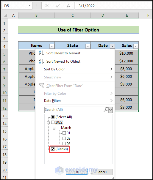
All rows containing blank cells will be filtered.
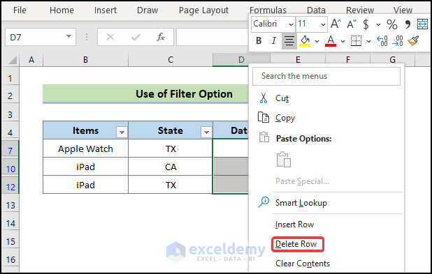
Select all rows, right-click, and choose Delete Row.

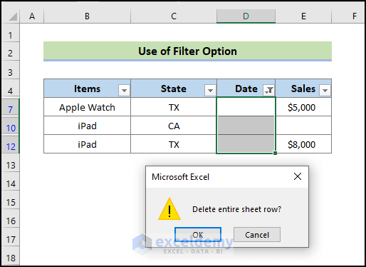
Confirm the row deletion in the Microsoft Excel message box.

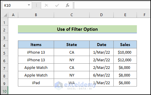
Withdraw the filter by pressing Ctrl + Shift + L again.

Method 3 – Applying Advanced Filter Feature to Eliminate Unused Cells

Steps:

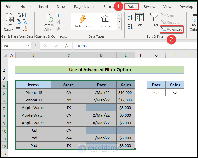
Enter the not equal to (<>) symbol in Cell G5 and H5.
Go to the Data tab and select Advanced.

In the Advanced Filter dialog, choose Copy to another location.
Specify List range (B4:E12), Criteria range (G4:H5), and Copy to (B14).

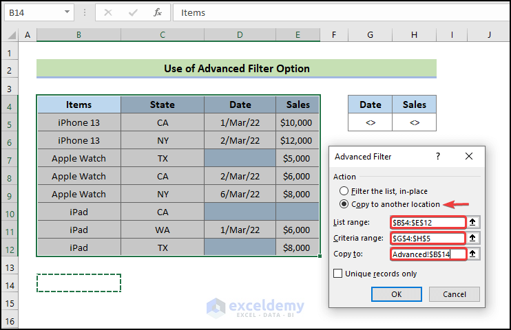
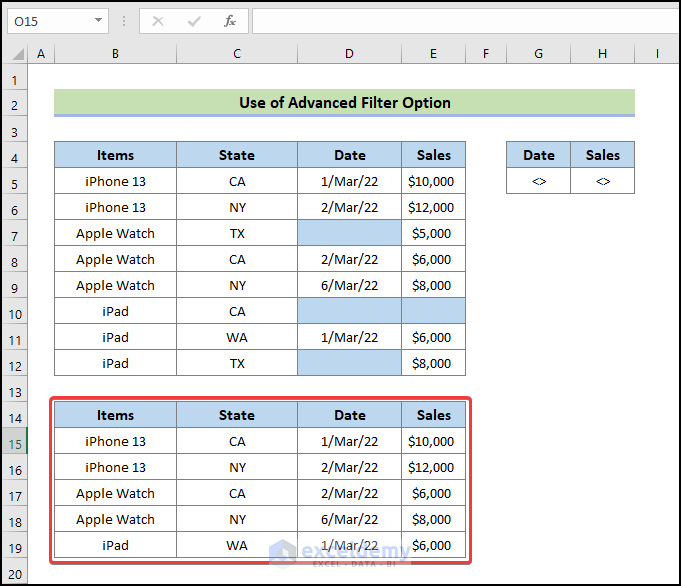
Press OK to filter the range to another location (empty cells deleted).

Method 4 – Remove Unused Blank Cells from a Vertical Range (Single Column)

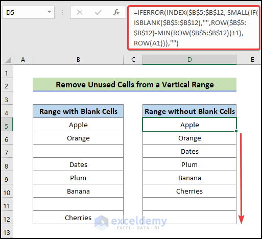
Use the following formula in Cell D5:

=IFERROR(INDEX($B$5:$B$12,SMALL(IF(ISBLANK($B$5:$B$12),"",ROW($B$5:$B$12)-MIN(ROW($B$5:$B$12))+1), ROW(A1))),"")

Press Enter.

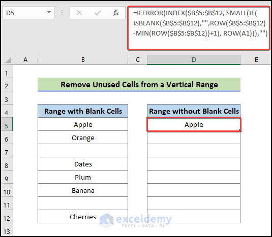
Drag down the Fill Handle icon to fill other cells with the formula.
The resulting range will exclude blank cells.

How Does the Formula Work?

ISBLANK($B$5:$B$12):
- The ISBLANK function checks whether a cell is blank or not in the range B5:E12 and returns either True or False.
- For example, if cell B5 is blank, it will return True; otherwise, it will return False.
ROW($B$5:$B$12):
- The ROW function returns the row numbers in the range B5:E12.
- The output is an array: {5;6;7;8;9;10;11;12} representing the row numbers.
MIN(ROW($B$5:$B$12)):
- The MIN function finds the lowest row number in the range, which is 5 in this case.
- The output is an array: {5}.
IF(ISBLANK($B$5:$B$12), “”, ROW($B$5:$B$12) – MIN(ROW($B$5:$B$12)) + 1):
- This formula combines the previous steps.
- It returns an array: {1;2;“”;4;5;6;“”;8}.
- The blank cells are replaced with an empty string (“”).
SMALL(IF(ISBLANK($B$5:$B$12), “”, ROW($B$5:$B$12) – MIN(ROW($B$5:$B$12)) + 1), ROW(A1)):
- The SMALL function returns the k-th smallest value from the array.
- In this case, it returns the smallest value (1) from the modified array.
- The reference to ROW(A1) ensures that it always returns the first value (k=1).
INDEX($B$5:$B$12, SMALL(…)):
- The INDEX formula returns the value from the B5:B12 range at the specified position (1 in this case).
- So, it returns “Apple” (assuming the value in B5 is “Apple”).
IFERROR(INDEX(…), “”):
- The IFERROR function wraps the INDEX formula.
- If the INDEX formula encounters an error (e.g., if there are no blank cells), it returns an empty string (“”).

Method 5 – Removing Unused Cells from a Horizontal Range

In contrast to the previous technique, we will now eliminate empty cells from a horizontal range of data. To achieve this, we’ll combine several Excel functions (IF, COLUMN, SUM, INDEX, and SMALL).

Enter the following formula in Cell C8:

=IF(COLUMN(B:B)<=SUM(--($B$5:$I$5<>""))+1,INDEX($B$5:$I$5,0,SMALL(IF($B$5:$I$5<>"",COLUMN($B$5:$I$5)-1,""),COLUMN(B:B)-1)),"")

Press Enter.

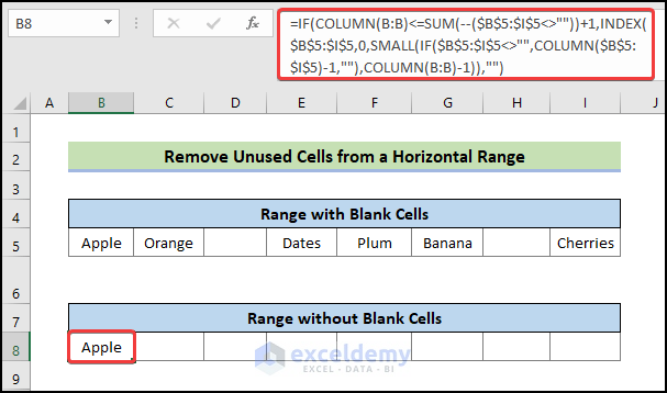
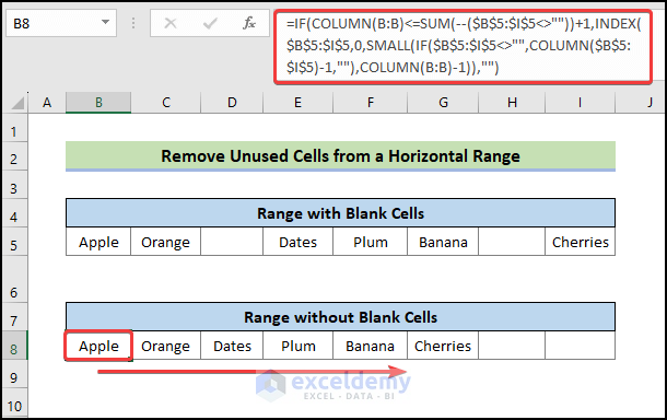
Drag the Fill Handle icon to the right to apply the formula to other cells.
You’ll notice that the resulting range does not include blank cells.

How Does the Formula Work?

COLUMN(B:B)<=SUM(–($B$5:$I$5<>””))+1

The above formula evaluates to: {TRUE}

Where, COLUMN(B:B) Returns the column number of B:B which is: {2}

$B$5:$I$5<>”” Evaluates to: {TRUE,TRUE,FALSE,TRUE,TRUE,TRUE,FALSE,TRUE}

SUM(–($B$5:$I$5<>””) Sums up the count of TRUE values and resulting in: {6}

INDEX($B$5:$I$5,0,SMALL(IF($B$5:$I$5<>””,COLUMN($B$5:$I$5)-1,””),COLUMN(B:B)-1))

The above formula returns: {“Apple”}

IF($B$5:$I$5<>””,COLUMN($B$5:$I$5)-1,””)

Here, the IF function checks whether $B$5:$I$5<>””, and replies accordingly: {1,2,””,4,5,6,””,8}

SMALL(IF($B$5:$I$5<>””,COLUMN($B$5:$I$5)-1,””),COLUMN(B:B)-1)

The SMALL function returns the k-th smallest value from our data range which is: {1}

IF(COLUMN(B:B)<=SUM(–($B$5:$I$5<>””))+1,INDEX($B$5:$I$5,0,SMALL(IF($B$5:$I$5<>””,COLUMN($B$5:$I$5)-1,””),COLUMN(B:B)-1)),””)

The above formula returns: {Apple}

Method 6 – Using the FILTER Function to Delete Unused Cells:

If you’re using Excel 365, you can eliminate empty cells using the FILTER function. Follow these steps:

Press Ctrl + T to create an Excel table from the data range (B4:E12).
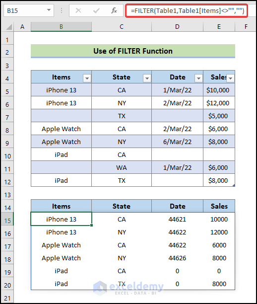
Enter the following formula in Cell B15:

=FILTER(Table1,Table1[Items]<>"","")

Press Enter.

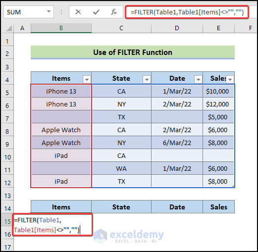
The array created by the formula will remove all blank cells from the first column (Items) of the table.

In the output image, you’ll see that rows with blank cells in the Items column have been removed, and empty cells in other columns are filled with a value of 0.

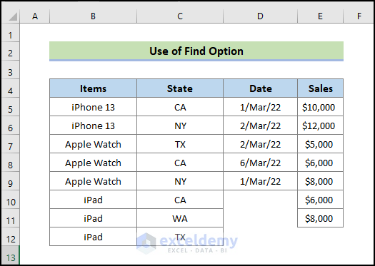
Method 7 – Using the Find Option to Delete Unused Cells

Follow these steps to accomplish the task:

Steps:

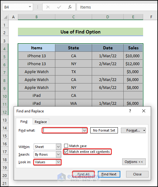
Select the range (B5:E12) of data.
Press Ctrl + F to open the Find and Replace dialog.
Leave the Find what field blank, choose Values from the Look in drop-down, and check Match entire cell contents.
Press Find All to get a list of blank cells.

Select the entire output (hold Ctrl key) and go to Home, select Cells, choose Delete and click on Delete Cells.

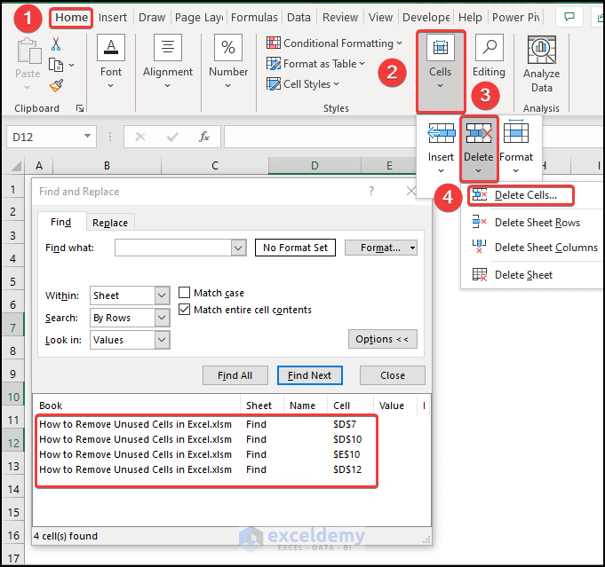
Press OK.

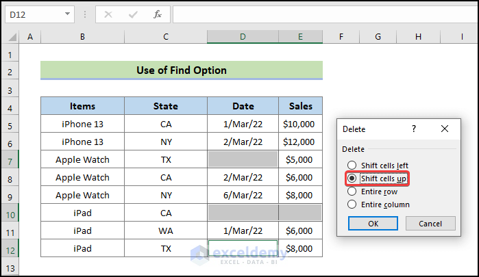
The resulting output will reflect the selected Shift cells up delete option.

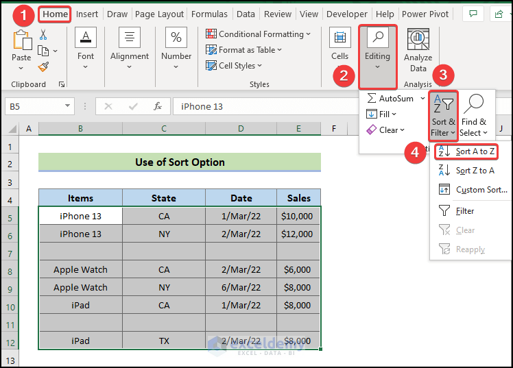
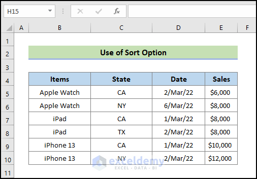
Method 8 – Using the Sort Command to Remove Unused Cells

In this method, we’ll demonstrate how to remove empty cells using the Sort option in Excel. Keep in mind that if you use this method, every row containing unused cells will be deleted.

Steps:

Select the range.
Go to Data, select Sort & Filter and click on the Sort A to Z icon.

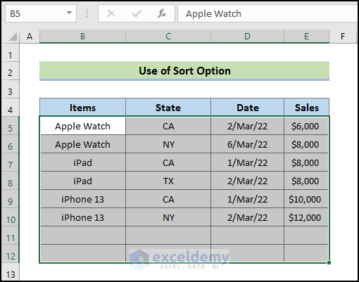
As a result, the data will be sorted, and at the end of the range, a list of all blank rows will be presented.

Press Ctrl + – from the keyboard to bring up the Delete dialog.
Choose the Delete Row option and press OK.

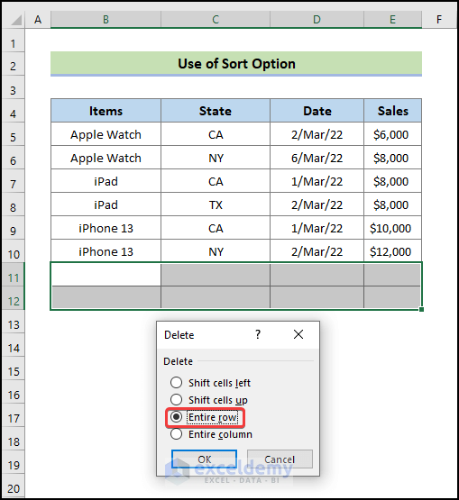
The final outcome will show that our data range has all the blank rows removed

Method 9 – Using Excel Power Query

Using Excel Power Query, we’ll demonstrate how to delete unused cells.

Steps:

Press Ctrl + T to create an Excel table from the data range.
Click anywhere in the table and go to Data and select From Table/Range.

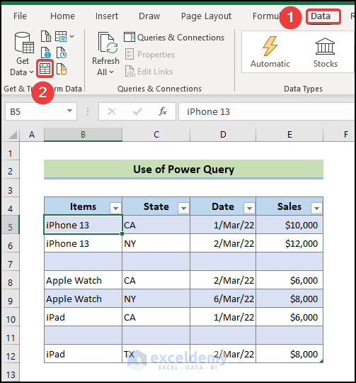
The table will appear in the Power Query Editor window, with null values in all blank cells by default.
Follow this path: Home, select Remove Rows and click on Remove Blank Rows.

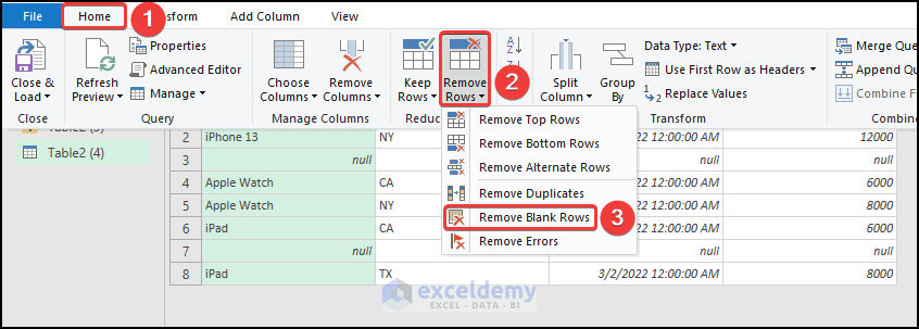
All rows containing null values will be removed.
To close the operation, go to Home, select Close & Load and click on Close & Load.

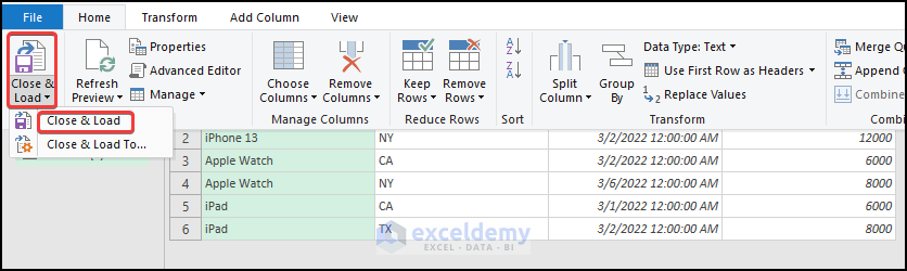
The final outcome will appear in a new Excel sheet.

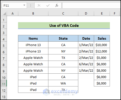
Method 10 – Applying VBA Code to Remove Unused Cells

We can also remove unused cells using Excel VBA code.

Steps:

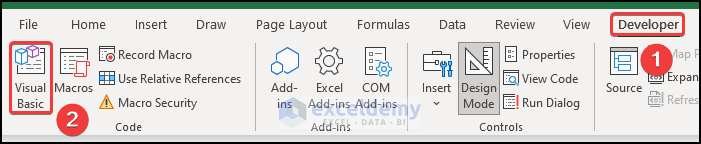
Open the VBA window by going to the Developer tab on your ribbon and selecting Visual Basic from the Code group.

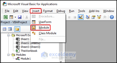
Insert a module for the code by going to the Insert tab in the VBA editor and clicking on Module from the drop-down.

Enter the following code in the new module:

Sub RemoveBlankCells()
    Dim rng As Range, cell As Range
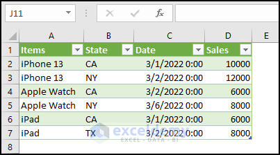
    Set rng = Range("B4:E12")
    For Each cell In rng
        If cell.Value = "" Then
            cell.Delete Shift:=xlShiftUp ' or Shift:=xlShiftToLeft
        End If
    Next cell
End Sub

Save the code.
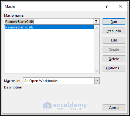
Close the Visual Basic window and press Alt + F8.
In the Macro dialogue box, select the macro and click Run.

The unused cells will be removed as shown below.

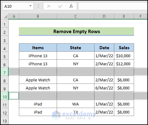
How to Remove Empty Rows in Excel

You can use the Context Menu to remove empty rows in Excel using the Delete command. Follow these steps:

Left-click on the mouse in the row number to select the empty row.
To select multiple rows, hold the CTRL key and select the row numbers.

Right-click on the mouse and from the Context Menu, choose Delete.

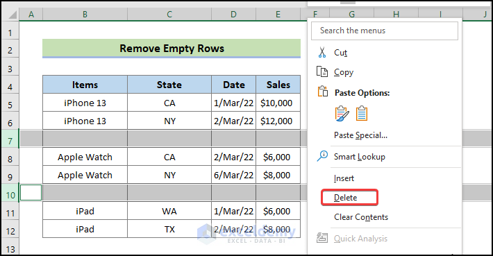
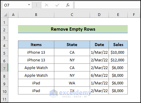
This will delete the selected empty rows.

Read More: How to Remove Blank Lines in Excel

Frequently Asked Questions

How to Delete Thousands of Blank Rows in Excel:

To remove blank rows from an Excel document, follow these steps:

Perform a “Find & Select” on the blank rows.
Select “Delete” from the Home tab.
Deleting rows or cells in Excel causes the data beneath them to move up.

How to Get Rid of Infinite Columns to the Right in Excel:

You can use the Excel context menu to delete infinite columns. Follow these steps:

Select the first column (e.g., column G) from where you want to delete infinite columns.
Press CTRL+SHIFT+RIGHT Arrow to select all columns to the right.
Excel will display the columns at the right end of your sheet, marked with gray color.
Right-click on any column header and choose Delete from the context menu.
The display will return to the beginning of the sheet, and the last column number of your Excel datasheet is AA.

How to Get Rid of Infinite Rows in Excel:

To remove infinite rows, use the Delete tab from the Home ribbon: