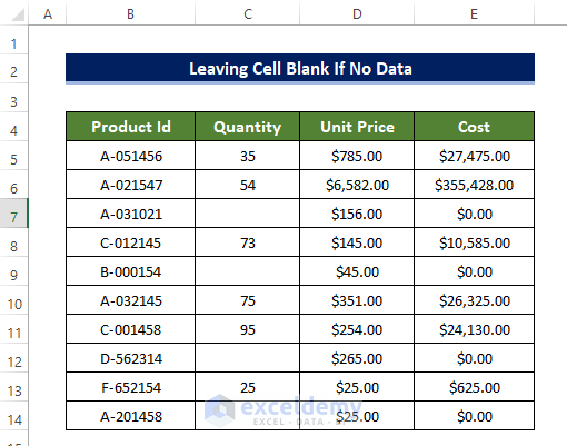
The sample dataset contains the columns Product ID, Quantity, Unit Price, and Cost columns where some of the values for quantity are missing. This leads to some entries in the column cost to be zero. We’ll modify the formula so that those cells lose the values.
Method 1 – Using the IF Function
Steps
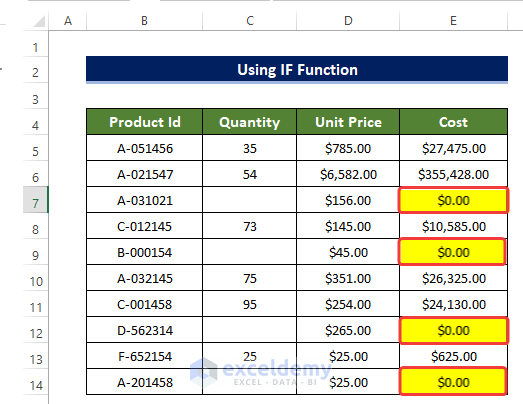
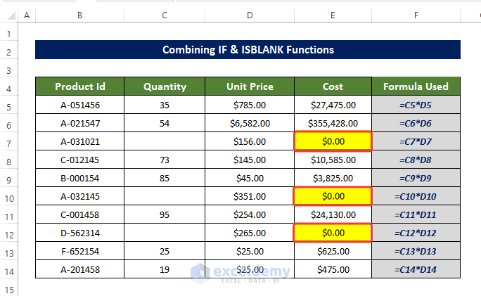
- The cells E7, E9 E12, and E14 are actually empty.
- The numerical value of those cells is equal to 0 and the cell formatting is expressing it as such.
- The formulas in the range of cells F5:F14 are shown below. These formulas force the cells to show zero values with the Currency format.
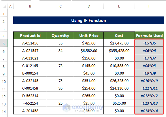
- Replace the formula in F5 with the following:
=IF(C5="","",C5*D5)
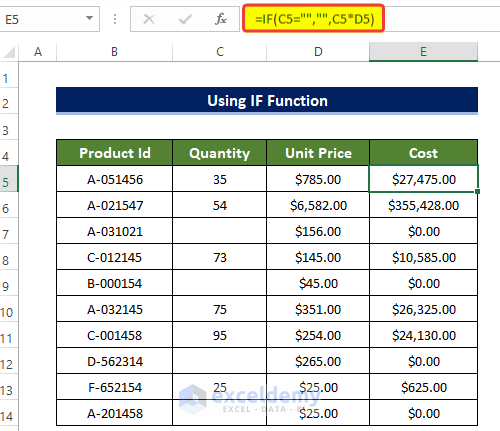
- Drag the Fill Handle to cell E14.
![]()
Read More: How to Ignore Blank Cells in Range in Excel
Method 2 – Combining IF and ISBLANK Functions
Utilizing the combination of IF and ISBLANK functions, we can find if the cell in Excel is Blank and then Leave it Blank if there is no data available for display.
Steps
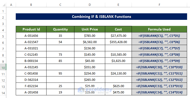
- The cells E7, E10, and E12 are empty. The formulas in the range of cells F5:F14 are shown below. Despite not having a value, these formulas force the cells to show zero values with Currency format.
- Replace the formula in F5 with the following:
=IF(ISBLANK(C5), "", C5*D5)
![]()
Formula Breakdown
- ISBLANK(C5): This function will check C5 cell is Blank or not. If it is Blank, then it will return a Boolean True. Otherwise, it will return a Boolean False.
- IF(ISBLANK(C5), “”, C5*D5): Depending on the return from the ISBLANK function, the IF function will return “”, if the return from the ISBLANK function is True. Otherwise, if the return from the ISBLANK function is False, the IF function will return the value of C5*D5.
- Drag the Fill Handle to cell E14.
Method 3 – Applying IF and ISNUMBER Functions
Steps:
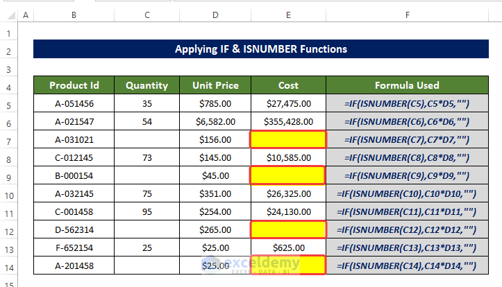
- The cells E7, E10, and E12 are empty. The formulas in the range of cells F5:F14 are shown below. Despite not having a value, these formulas force the cells to show zero values with Currency format.
![]()
- Replace the formula in F5 with the following:
=IF(ISNUMBER(C5),C5*D5,"")
![]()
Formula Breakdown
- ISNUMBER(C5): This function will check C5 cell is a number or not. If it is a number, then it will return a boolean True. Otherwise, it will return a Boolean False.
- IF(ISNUMBER(C5),C5*D5,””): Depending on the return from the ISNUMBER function, the IF function will return “”, if the return from the ISBLANK function is False. Otherwise, if the return from the ISNUMBER function is True, IF function will return the value of C5*D5.
- Drag the Fill Handle to cell E14.
Note
- The ISNUMBER will return True only f the entry is Number. For any form of non-numerical value, like Blank, space, etc., the ISNUMBER will return False.
- So, the formula here will make the cell Blank whether the cell content is Blank or other non-numerical characters. Users need to be aware of this.
Method 4 – Using Custom Formatting
Custom formatting will help us to select individual cells and then format them Leave only the Blank cells if there is no other data available for display.
Steps
- The cells E7, E10, and E12 are empty. The formulas in the range of cells F5:F14 are shown below. Despite not having a value, these formulas force the cells to show zero values with Currency format.
![]()
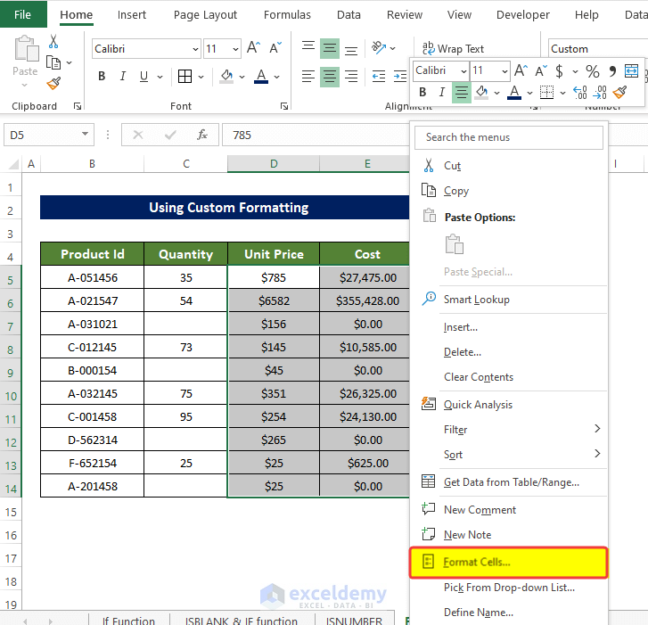
- Select the range of cells D5:F14.
- Right-click on the range.
- From the context menu, click on Format Cells.
- In the Format Cells dialog box, click on Custom from the Number tab.
- Type “$General;;” in the Type field and then click OK.
![]()
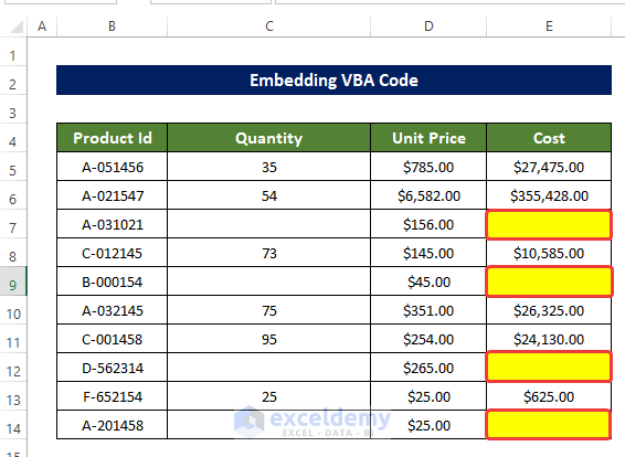
- The values without data show up as blank.
![]()
Note
- In the custom formatting dialog box, we need to type “;;” after General. We also need to put a $ sign in front of the General to keep the Currency format.
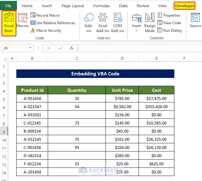
Method 5 – Embedding VBA Code
Steps
- Go to the Developer tab, then click Visual Basic.
- Click Insert and select Module.
![]()
- In the Module window, enter the following code.
Sub Blank_Cell()
Dim x As Range
For Each x In Range("B5:F14")
If x.Value = 0 Then x.Value = " "
Next x
End Sub![]()
- Close the window.
- Go to the View tab and select View Macros.
![]()
- Select the macro that was created just now. The name we used is Blank_Cell.
- Click Run.
![]()
- The cells without the data now show a Blank cell instead of $0.
Download the Practice Workbook
Related Articles
- How to Delete Blank Cells and Shift Data Up in Excel
- How to Remove Blank Cells in Excel
- How to Remove Blank Lines in Excel
- How to Delete Blank Cells and Shift Data Left in Excel
- How to Remove Unused Cells in Excel
- How to Remove Blank Cells from a Range in Excel
<< Go Back to Excel Cells | Learn Excel
Get FREE Advanced Excel Exercises with Solutions!

My preference was to use the formatting method, less messing around, nice output – I can fill the calculation in for the entire column, and any zero figures will disappear. However, unfortunately it also hides negative numbers which isn’t ideal in some circumstances!
Hello, OZTIMS!
Thanks for sharing your problem with us!
Instead of using this format ($General;;), you can use the ($0;-0;;@). This will keep the negative values. To use this follow method-4.
1. When the Format Cells dialog box will appear, go to Number > Custom.
2. Type $0;-0;;@ in the Type field.
3. Finally, click OK.
4. Now, if you see the result, this will also show a negative number. The cell will only be blank if the cell has no data.
Hope this will help you.
Good Luck!
Regards,
Sabrina Ayon
Author, ExcelDemy.
at first it appeared complicated but this was easy to follow.
Dear Alex,
Thanks for your feedback.
Regards
Exceldemy
Thanks for a great article!
How do you leave a blank cell, as apposed to “$N/A”, when you are using index and match function.
My cell currently has the formula: =INDEX(‘Round 1′!$B$3:$AJ$25,MATCH(A5,’Round 1’!$B$3:$B$25, 0),34).
Not all of the “matches” will be found on each worksheet (it is a scoresheet and not all individuals compete each round), and therefore return the $N/A.
Thanks!
Hello Lory,
You can use the following formula: =IFERROR(INDEX(‘Round 1′!$B$3:$AJ$25,MATCH(A5,’Round 1’!$B$3:$B$25, 0),34),””)
It will leave a cell blank if no matches are found.
Regards
ExcelDemy