Scenario
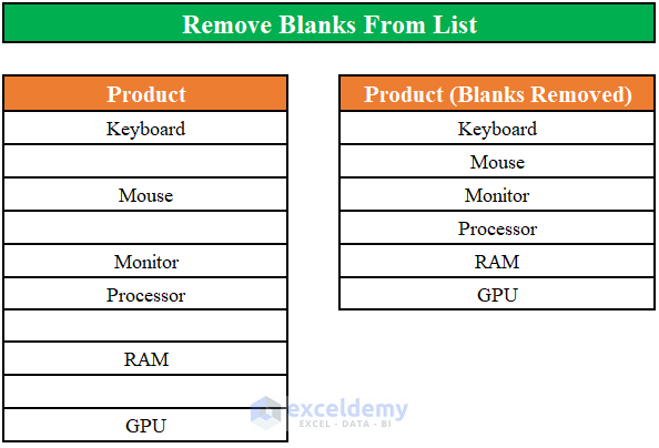
Let’s consider a scenario where we have an Excel worksheet containing a list of various computer hardware and accessories. Unfortunately, this list contains several blank spaces. Our goal is to remove these blanks using formulas in Excel.
Method 1 – Removing Blanks from a Vertical List in Excel Using an Array Formula
Step 1
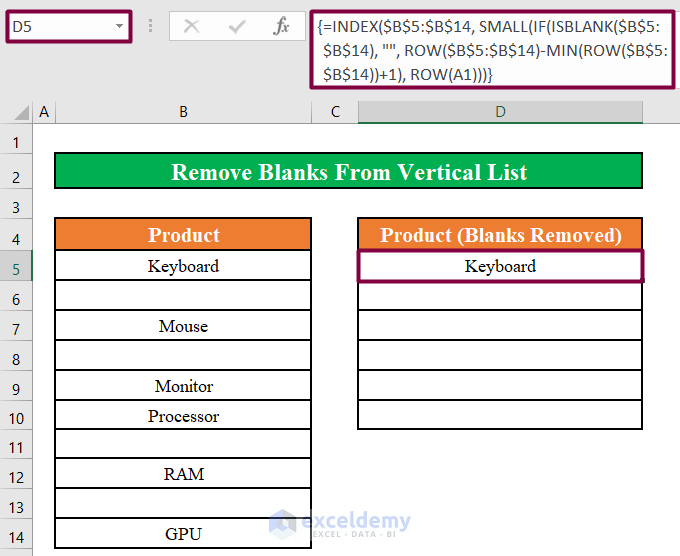
- In cell D5, enter the following array formula:

- Press ENTER and the formula will return the first non-blank item from the list.
Step 2
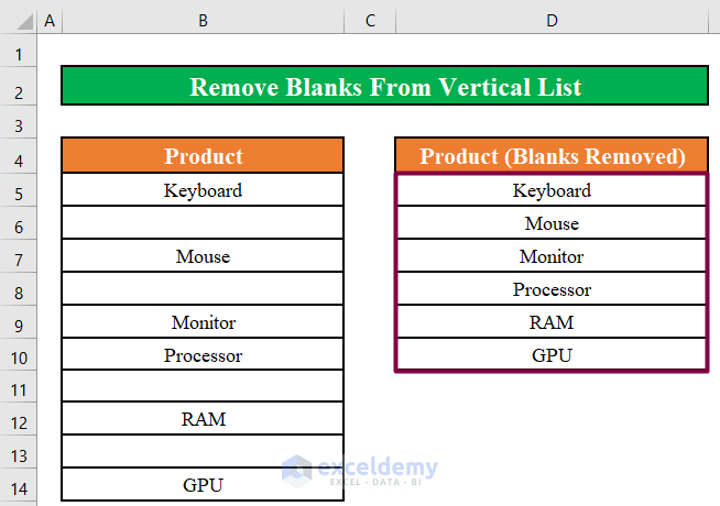
- Drag the fill handle of cell D5 to apply the formula to the remaining cells.
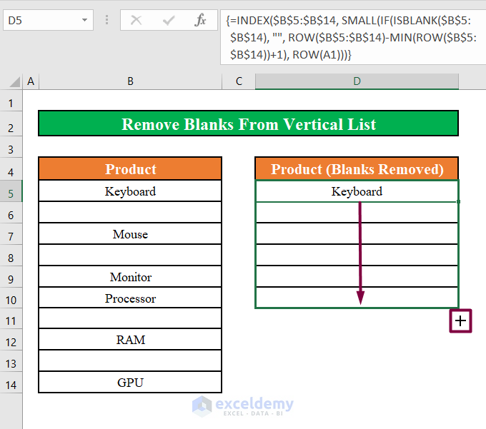
- You’ll now have a list of all products without any blank cells.
Read More: How to Set Cell to Blank in Formula in Excel (6 Ways)
Method 2 – Removing Blanks from a Horizontal List Using an Array Formula
Alternatively, we can use another array formula to remove blank cells from a horizontal list. Follow the steps below:
Step 1
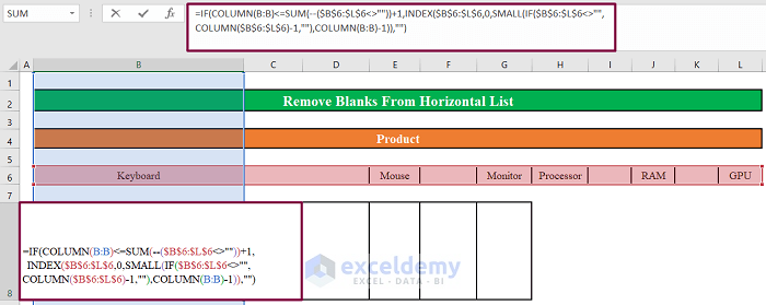
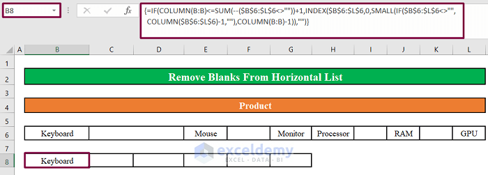
- In cell B8, enter the following array formula:
=IF(COLUMN(B:B)<=SUM(–($B$6:$L$6<>””))+1,INDEX($B$6:$L$6,0,SMALL(IF($B$6:$L$6<>””,
COLUMN($B$6:$L$6)-1,””),COLUMN(B:B)-1)),””)
Formula Breakdown
- IF function allows logical comparisons.
- SUM function adds all the numbers in a range of cells.
- INDEX returns the value of an element in an array.
- SMALL finds the k-th smallest value in a dataset.
- COLUMN returns the column number of a reference.
- MIN extracts the lowest value from a range of cells or references.
- Press ENTER and the formula will return the first non-blank item from the list.
Step 2
- Drag the fill handle of cell D5 horizontally to apply the formula to the remaining cells.
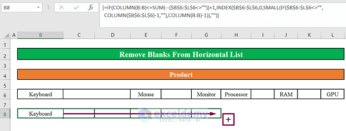
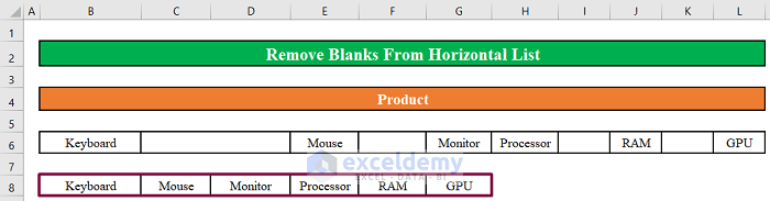
- You’ll now have a list of all products without any blank cells.
Read More: Find, Count and Apply Formula If a Cell is Not Blank (With Examples)
Similar Readings
- How to Delete Blank Cells in Excel and Shift Data Up
- Apply Conditional Formatting in Excel If Another Cell Is Blank
- How to Ignore Blank Cells in Range in Excel (8 Ways)
- If Cell is Blank Then Show 0 in Excel (4 Ways)
- How to Calculate in Excel If Cells are Not Blank: 7 Exemplary Formulas
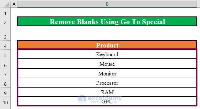
Method 3 – Using the “Go To Special” Option to Remove Blanks from the List
The easiest and most efficient way to remove blanks from a list is to use the “Go To Special” menu. Follow these steps:
Step 1
- Go to Home, select Editing, click on Find & Select and click on Go to Special. This feature allows you to find and select cells based on their content.
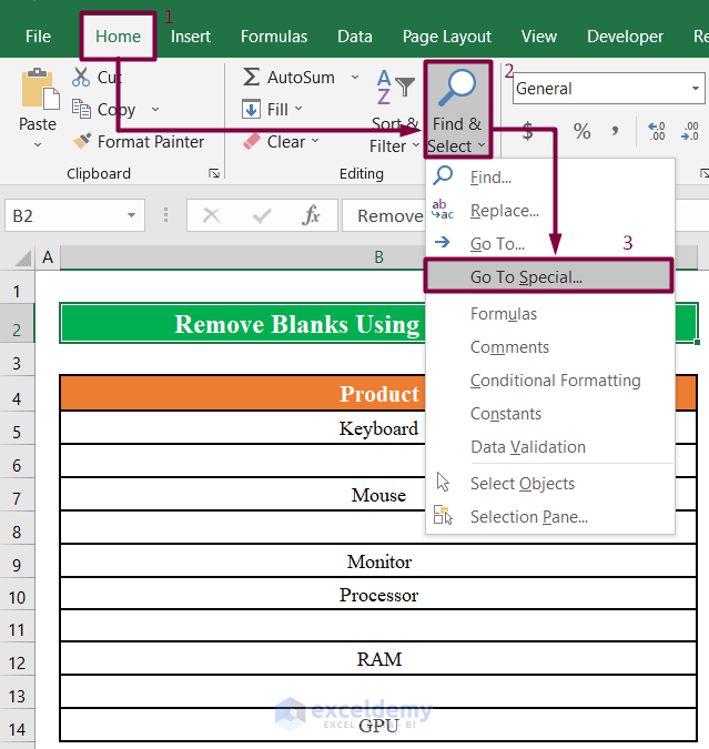
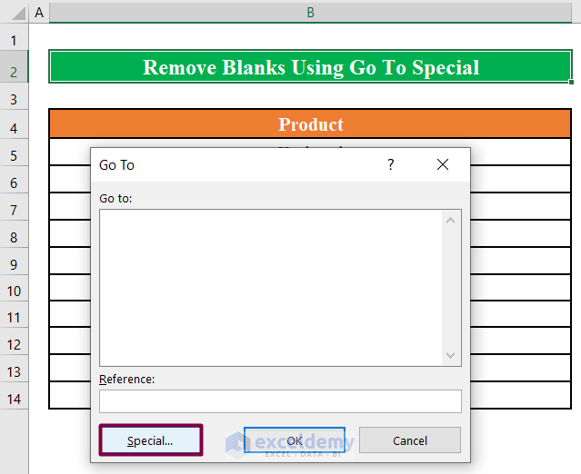
- Alternatively, press the F5 key to open the Go To menu, then click the Special button in the lower-left corner.
Step 2
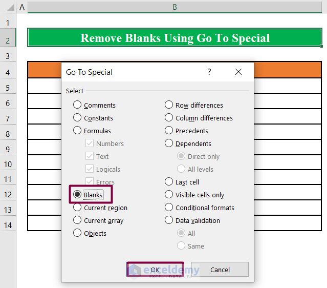
- Select Blanks from the Go To Special dialog.
- Click OK.
Step 3
- Under the Home tab, click the Delete drop-down menu.
- Choose Delete Cells from the menu.
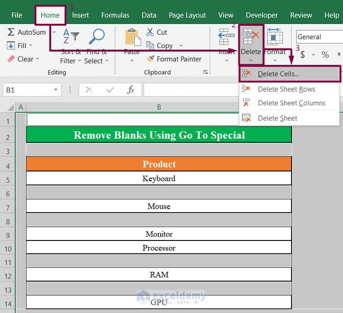
- In the Delete dialog, select Shift cells up.
- Click OK.
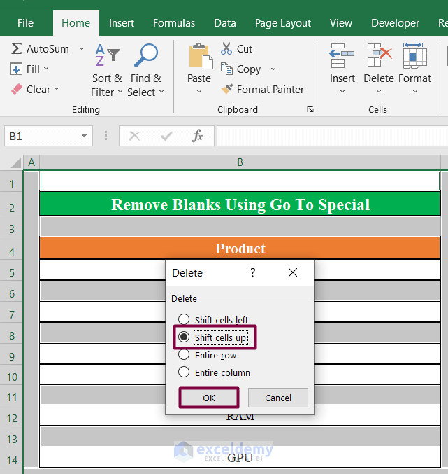
- You’ll now have a list of all products without any blank cells.
Read More: How to Fill Blank Cells with Value Above in Excel
Method 4 – Removing Blanks from a List Using the COUNTBLANK Function
Another approach to remove blanks from the list involves using the COUNTBLANK function in conjunction with table filtering. Let’s walk through the steps:
Step 1
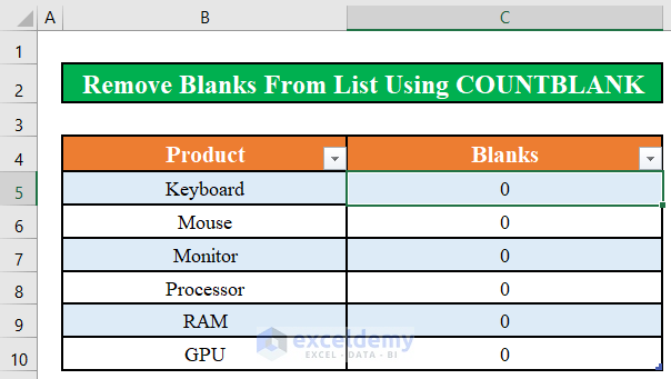
- In cell D5, enter the following formula:
=COUNTBLANK(B5)
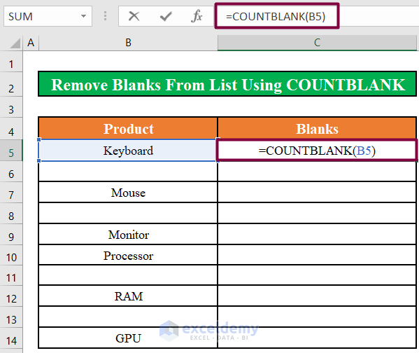
Formula Breakdown
The COUNTBLANK formula counts the blank cells within the specified range.
- Press ENTER and you’ll see that the formula returns zero (0) because cell B5 contains the text Keyboard, not a blank value.
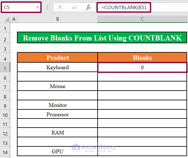
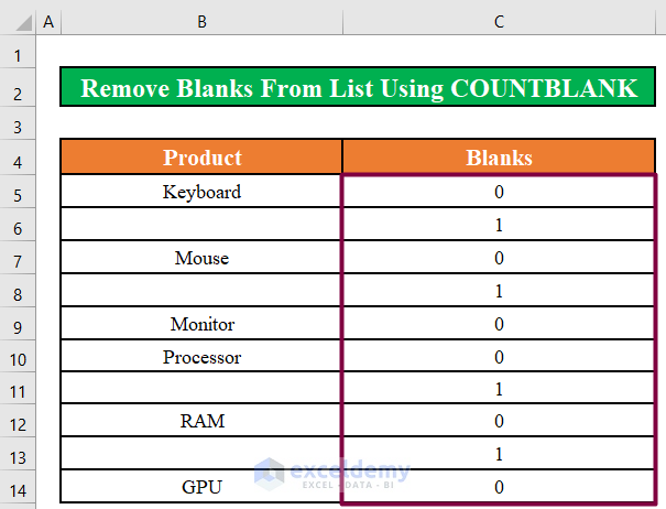
Step 2
- Drag the fill handle of cell C5 downward to apply the formula to the remaining cells.
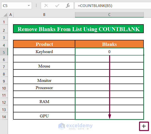
- The formula will return zero (0) for cells containing text and one (1) for empty cells in the Product column.
Step 3
- Select all cells in the data range, including the column header.
- Under the Insert ribbon, choose Table.
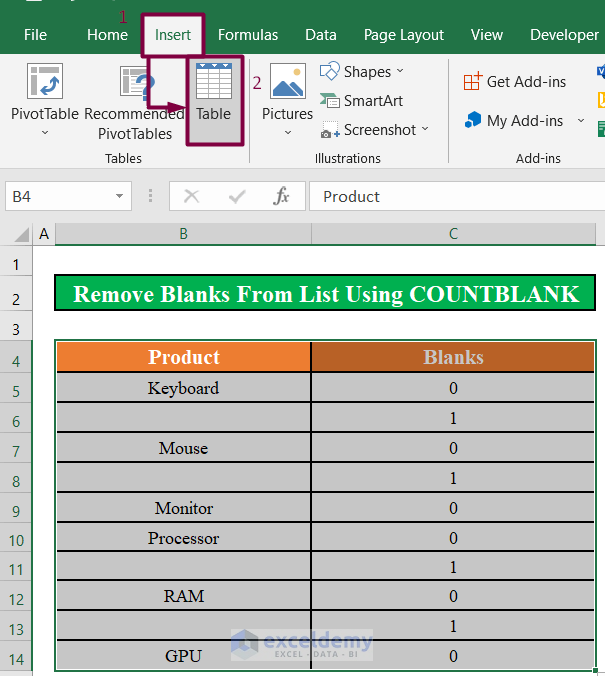
- In the Create Table window, select the My table has headers option and click OK.
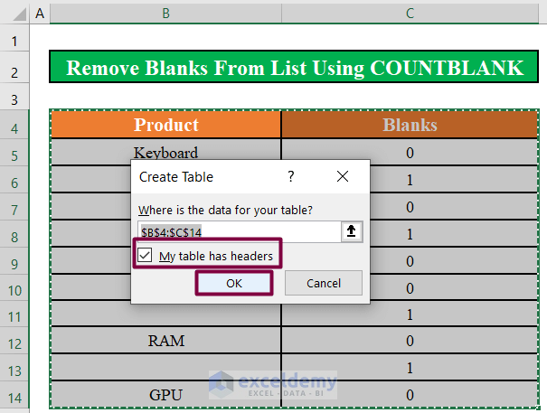
- Your data range will now be formatted as a table, with a Filter icon displayed for each column.
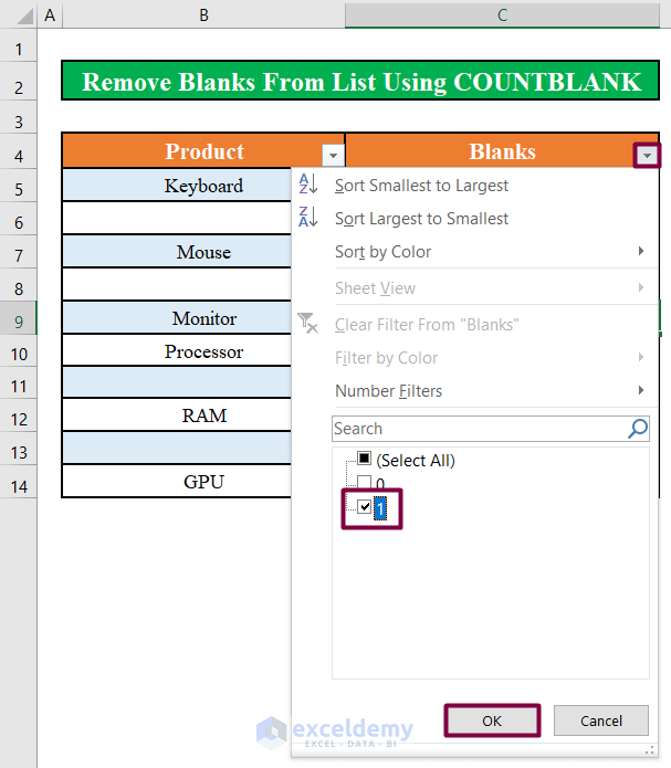
- Click the Filter icon for the Blanks column.
- Select only the value 1 (representing blank cells).
- Press OK.
Step 4
- You’ll now see only the empty cells.
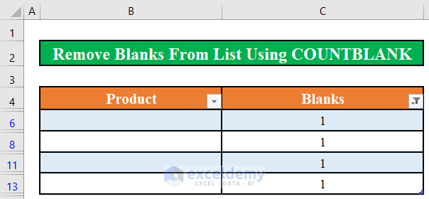
- Select the entire data range.
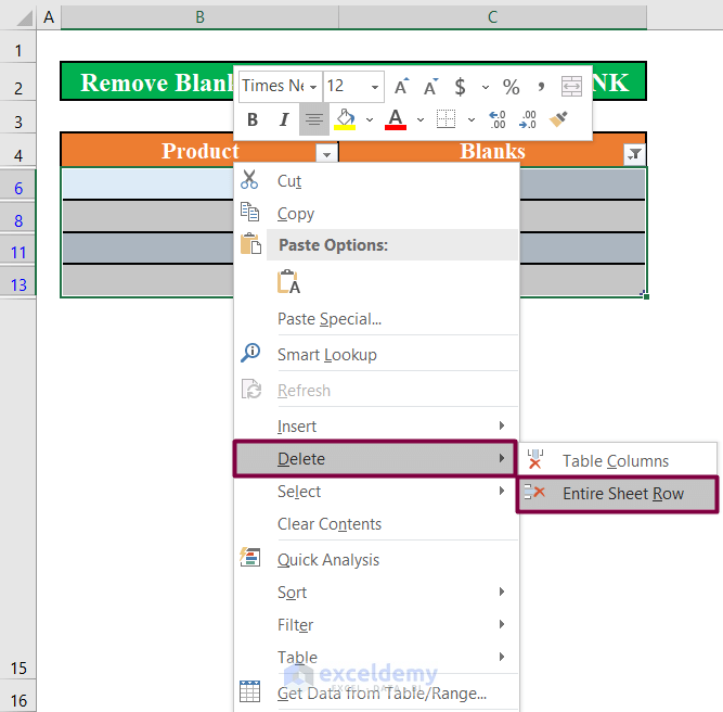
- Right-click any cell in the Blanks column to access the Context Menu.
- Go to Delete and click on Entire Sheet Row to remove all blank rows.
- Clear the filter by selecting the filter icon and choosing Clear Filter From “Blanks”.
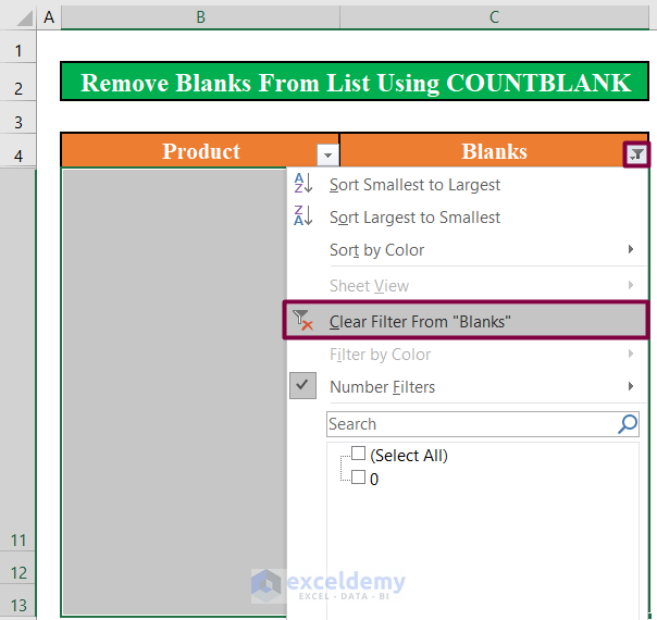
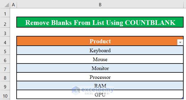
- You’ll now see only rows containing text in the Product column.
Additionally, if you want to make your dataset smaller, you can remove the blank column:
- Right-click any cell in the Blanks column.
- Click Delete and select Table Columns.
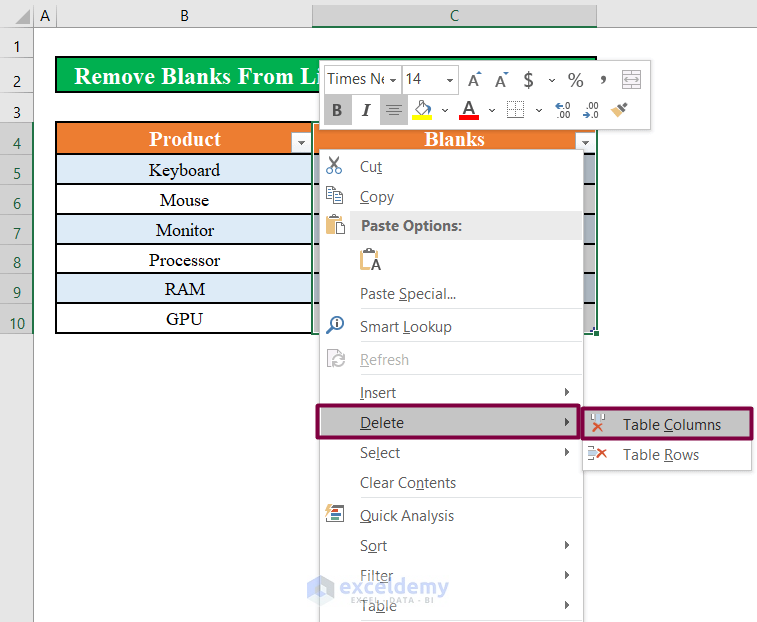
- You’ve successfully removed all blanks from the list.
Read More: How to Delete Empty Cells in Excel (6 Methods)
Quick Notes
Array Formulas
- The formulas used are array formulas. To insert them in a cell, press CTRL+SHIFT+ENTER together, and they will be enclosed in curly braces.
- These formulas efficiently handle blank cells in your data.
Removing Blanks in Excel
- If you’re interested in removing blank spaces in Excel, consider reading the linked article.
- Additionally, learn how to add blank spaces in Excel from another resource.
Download Practice Workbook
You can download the practice workbook from here:
Related Articles
- How to Remove Blank Cells from a Range in Excel (9 Methods)
- Make Empty Cells Blank in Excel (3 Methods)
- How to Deal with Blank Cells That Are Not Really Blank in Excel (4 Ways)
- Fill Blank Cells with 0 in Excel (3 Methods)
- Null vs Blank in Excel
- How to Delete Empty Cells in Excel (8 Easy Methods)


Hi – I tried this and at first all I got in the cell with the formula was the #NAME error. I double-clicked the cell to mess around with the formula, changed nothing, hit enter, and then it worked for the first item. When I propagated the formula, though, every other cell returned an error: #NAME? or #NUM!. It would be AMAZINGLY AWESOME to get this formula to work because there are many situations where I would love to have a formula that automatically updates and removes blank lines from a series of cells but I have no idea how to fix it. Here is the formula I put into my worksheet:
=INDEX($C$8:$C$55, SMALL(IF(ISBLANK($C$8:$C$55), “”, ROW($C$8:$C$55)-MIN(ROW($C$8:$C$55))+1), ROW(A1)))
My data are in column C from C8 to C55. They are:
C8 = Housing
C9-C11 = blank
C12 = Vehicles
C13-15 = blank
C16 = Gas
C17 = blank
C18 = Utilities
C19-23 = blank
C24 = Food
C25-27 = blank
C28 = Party
C29 = blank
C30 = Saving
C31-33 = blank
C35 = Carl
C35-38 = blank
and so on. I can add more if you need it.
To be fair, although I have minor experience with coding (C++ and Python), INDEX functions in Excel are like hieroglyphics to me; I just don’t get it. What am I doing wrong? Why will it work for the first cell but when I propagate (drag the fill button as it says above) does it stop working?
Hello, TRYSTAN! Can you please email us your Excel file containing the dataset with the problem? Thanks.
Why not use the FILTER function? Perhaps combined with the UNIQUE function?
=UNIQUE(FILTER(B5:B14,B5:B14″”))
Hello NK,
It’s awesome that you have found another solution which is applicable by adding a simple symbol in the formula you have mentioned. Yes obviously it is possible to remove blank from lists using the combination of UNIQUE and FILTER functions. The formula should be for the dataset of this article.
=UNIQUE(FILTER(B5:B14,B5:B14<>“”))
You need to add the symbol <> extra.
Here, the FILTER function is used to remove any blank values from the data.
The <> symbol is a logical operator that means does not equal.
The filtered data is returned directly to the UNIQUE function as the array argument. The UNIQUE function then removes duplicates and return the final array.
Thanks with Regards,
Towhid
Excel & VBA Content Developer
Here is a Better Formula:
=FILTER($B$5:$B$14,LEN($B5:$B14)>0)
Hello Frank,
Thanks for your suggestion. It’s the beauty of Excel it provides better formula with updated functions. FILTER function is one of the most dynamic and useful function. Keep contributing Excel tips with ExcelDemy!
Regards
ExcelDemy
It took me some times to realize that ISBLANK returns FALSE for a cell containing an equal sign and two double quotes ( =”” ) which, to me, means an empty line. So I replaced ISBLANK($B$5:$B$14) by ($B$5:$B$14)=”” and it works for me.
Hello Patrick Raimond,
Great observation! Yes, it can be a bit confusing, ISBLANK only returns TRUE if a cell is truly empty, not if it contains a formula like =””.
In those cases, checking = “” directly, as you did, is the best approach. Thanks for sharing your solution, this tip will definitely help others who run into the same issue!
Regards
ExcelDemy