How to Find Blank Cells in Excel (8 Easy Ways)

Method 1 – Use Go To Special Dialogue Box to Find Blank Cells in Excel

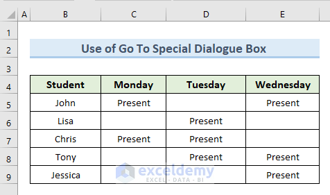
In the below screenshot, we have the attendance of 6 students for 3 days. We can see their attendance status as Present. The blank cell means that the student was absent on that day. We’ll use to “Go to Special” method to find the blank cells in this dataset.

STEPS:

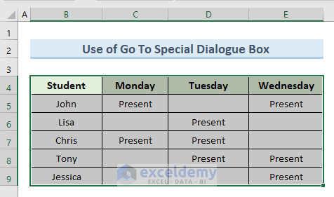
• Select the cell range (B4:E9).

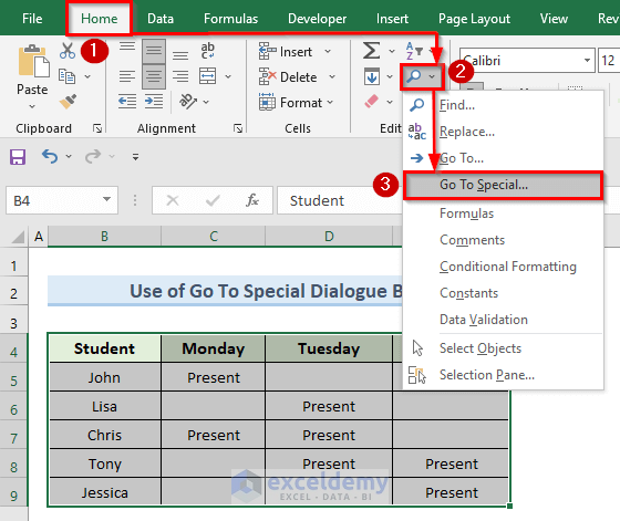
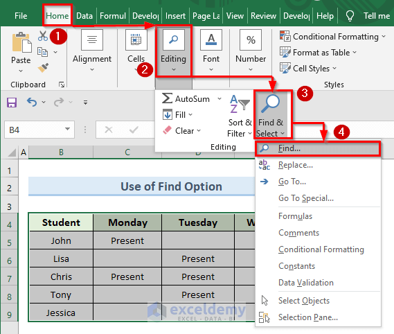
• Go to the Home tab.
• Select the option “Find & Select” from the Editing section of the Excel ribbon.
• Choose “Go To Special” from the drop-down.

• Check the Blanks option and press OK.
• Alternatively, you can use a keyboard shortcut to perform the above methods. Press Ctrl + G to open the “Go-To” dialogue box. Next press Alt + S to open the “Go To Special” dialogue box before using Alt + K to check the Blanks option.

• You can now see that the above command finds and selects all the blank cells in the cell range (B4:B9).

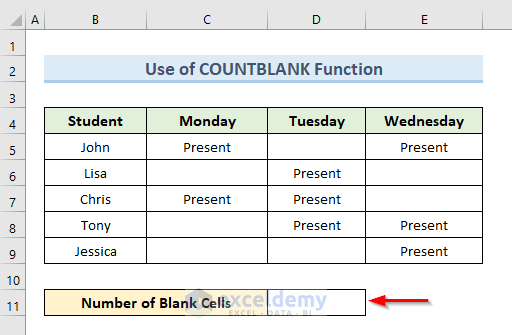
Method 2 – Use Excel COUNTBLANK Function to Find Blank Cells

The COUNTBLANK function is classified as a statistical function in Excel. COUNTBLANK is a function that finds and counts the number of blank cells in a range of cells. To illustrate this method we will continue with the same dataset that we used in the previous method but we will return the number of blank cells in cell D11.

STEPS:

• Select cell D11.
• Insert the following formula in that cell:

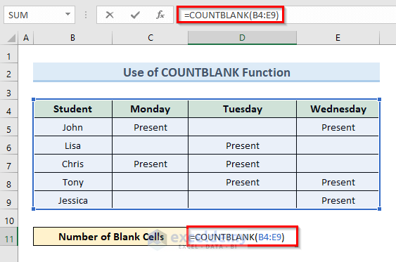
• Press Enter.
• The above command returns value 7 in cell D11. This means there are 7 blank cells in the cell range (B4:E9).

Method 3 – Find Blank Cells with Excel COUNTIF Function

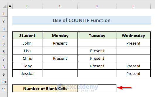
The COUNTIF  function is also a statistical function. It generally counts cells that satisfy a specific criterion. To illustrate this method we will use the same dataset that we used before.

STEPS:

• Select cell D11.
• Write down the following formula in that cell:

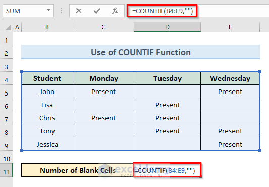
• Press Enter.
• You’ll get the number of blank cells 7 in cell D11.

Read More: How to Find & Count If a Cell Is Not Blank

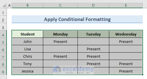
Method 4 – Apply Excel Conditional Formatting to Highlight Blank Cells

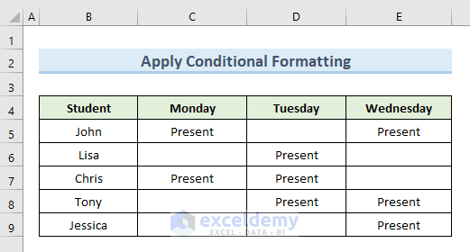
“Conditional Formatting” is used to apply formatting to a cell or range of cells. In this example, we will highlight blank cells from the dataset that we used in the previous article.

STEPS:

• Select the cell range (B4:E9).

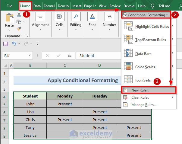
• Go to the Home tab.
• Click on the option “Conditional Formatting” from the ribbon.
• From the drop-down menu select the option “New Rule”.

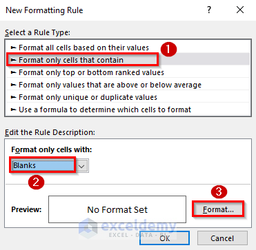
• You’ll see a new dialogue box named “New Formatting Rule”.
• From the “Select a Rule Type” section, choose the option “Format only cells that contain”.
• Select the option Blanks in the “Format only cells with”section.
• Click on Format.

• The “Format Cells” dialog box will appear.
• Go to Fill
• Select any fill color from the available colors and press OK.

• The above action gets us back to the “New Formatting Rule” dialog box.
• Use the Preview box of the Format option to see the newly added fill color.
• Press OK.

• You can now see that all the blank cells in the cell range (B4:E9) are highlighted.

Read More: How to Highlight Blank Cells in Excel

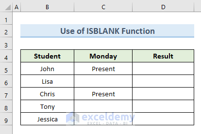
Method 5 – Identify Blank Cells with ISBLANK Function in Excel

The ISBLANK function is considered an information function. This function checks whether a cell is blank or not. It returns TRUE if a cell is blank and FALSE if the cell is non-blank. We are using the following dataset for this example which is slightly modified from the previous one.

STEPS:

• Select cell D5.
• Input the following formula in that cell:

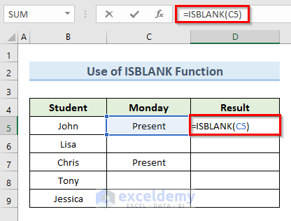
• Press Enter.
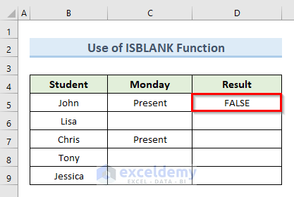
• We get the value FALSE in cell D5 as cell C5 is not blank.

• Select cell D5 again.
• Drop the mouse pointer to the selected cell’s bottom right corner, where it will convert into a plus (+) sign, as shown in the image below.
• Copy the formula of cell D5 into the other cells by clicking on the plus (+) sign and dragging the Fill Handle down to cell D10. You can also double-click on the plus (+) sign to get the same result.

• Release the mouse click.
• You can see the above action returns TRUE if the cell is blank and FALSE if the cell is non-blank.

Method 6 – Detect Blank Cells Using Find Option

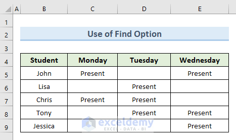
We can also find blank cells of a dataset by using the Find option from the Excel ribbon. To illustrate this method we will use the following dataset. You can take a look at the below screenshot of the dataset.

STEPS:

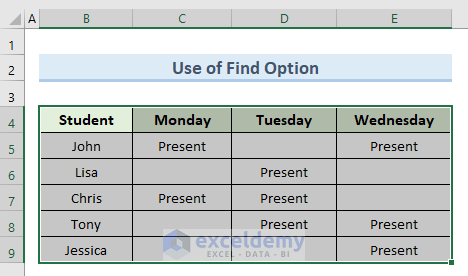
• Select the cell range (B4:E9).

• Go to the Home tab.
• Select the option “Find & Select” from the Editing section of the ribbon.
• From the drop-down select the option Find

• A new dialog box named “Find and Replace” will appear.
• In that box, set the following values for the mentioned options:

Find what: Keep this box blank.

Within: Select the option Sheet.

Search: Select the option “By Rows”.

Look in: Select the option Values.

• Click on “Find All”.

• You can see the list of all blank cells from the selected range (B4:E9).

Method 7 – Apply an Excel Filter to Find Blank Cells from Specific Column

You can use the Filter option to find blank cells for a specific column. This method is not perfect for finding blank cells from any particular data range. To explain this method we will continue with the dataset that we used in the previous example.

STEPS:

• Select the cell range (B4:E9).
• Go to the Home tab.
• Select the option Filter from the “Sort & Filter” section of the Excel ribbon.

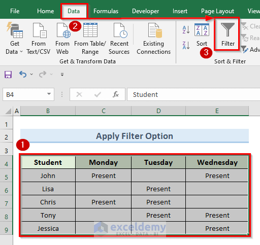
• The above command applies a filter to the selected data range. We can see the filter icons in the header cells.

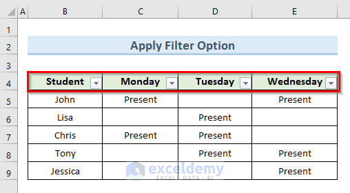
• Click on the filtering icon of cell C4 with the value Monday.
• Check the Blanks option from the menu.
• Press OK.

• You can now only see the blank cells in column C.

NOTE:

This method finds blank cells for individual columns instead of the whole data range. So, if we want to find the blank cells from the column with the heading Tuesday we have to filter this column individually for blank cells like the previous example.

Method 8 – Discover the First Blank Cell in a Column

Method 8.1. – Spot the First Blank Cell in  a Column with a Formula

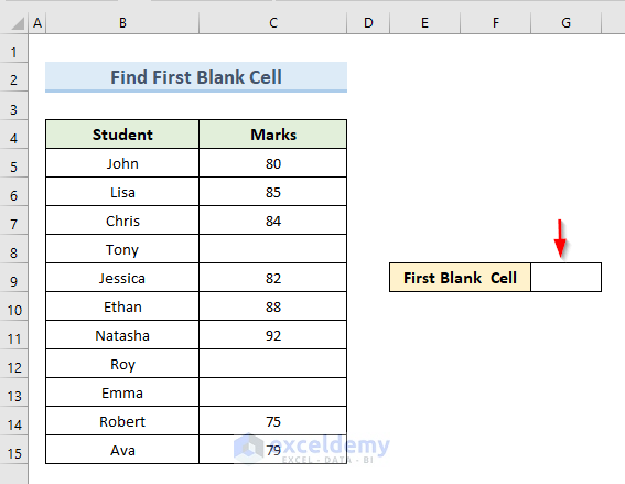
In this method, we will use a formula to find the first blank cell from a column. We have given a screenshot below of our dataset. There are blank cells in column C. We will find the first blank cell from that column and will return the cell number in cell G9.

STEPS:

• Select cell G7.
• Insert the following formula in that cell:

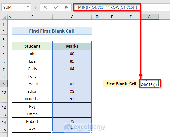
• Press Enter if you are using Microsoft Excel 365. Otherwise press Ctrl + Shift + Enter.
• You can see that the row number of the first blank cell is 8.

How Does the Formula Work?

• IF(C4:C15=””,ROW(C4:C15)): This part finds out the row numbers of all blank cells in range (C4:C15).
• MIN(IF(C4:C15=””,ROW(C4:C15))): From all the row numbers of blank cells, this part returns the minimum row number 8 which is also the first blank cell.

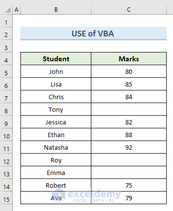
Method 8.2 – Use VBA Code to Find the First Blank Cell

The use of VBA (Visual Basic for Application) code is another convenient way to find the first blank cell in Excel. To explain this method we will continue with our previous dataset.

STEPS:

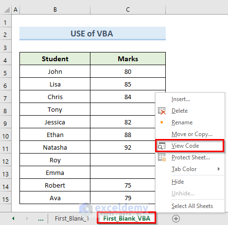
• Right-click on the active sheet.
• Click on the option “View Code” from the available options to open a blank VBA module.

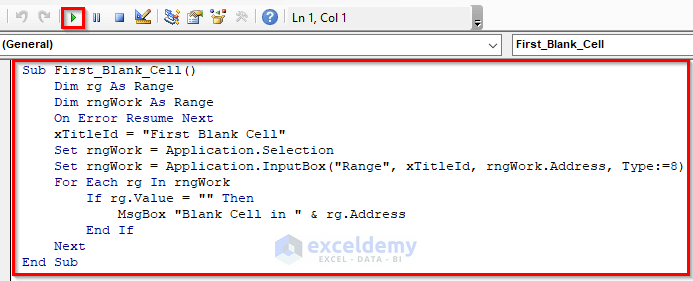
• Insert the following code in the blank module:

Sub First_Blank_Cell()
Dim rg As Range
Dim rngWork As Range
On Error Resume Next
xTitleId = "First Blank Cell"
Set rngWork = Application.Selection
Set rngWork = Application.InputBox("Range", xTitleId, rngWork.Address, Type:=8)
For Each rg In rngWork
If rg.Value = "" Then
MsgBox "Blank Cell in " & rg.Address
End If
Next
End Sub

• Click on Run or press F5 to run the code.

• A new dialogue box will appear. Go to the input box named Range and insert the data range value ($B4:$C$15).
• Press OK.

• A message box shows us that the cell number of the first blank cell is $C$8.

Download Practice Workbook

You can download the practice workbook from here.

Related Articles

• How to Make Empty Cells Blank in Excel
• How to Deal with Blank Cells That Are Not Really Blank in Excel
• Return Non Blank Cells from a Range in Excel
• Null vs Blank in Excel
• How to Set Cell to Blank in Formula in Excel
• Formula to Return Blank Cell instead of Zero in Excel

<< Go Back to Excel Cells | Learn Excel