The easiest way to to return a blank cell instead of zero in Excel is to use a formula. In this article we’ll demonstrate and explain that formula, and provide 5 alternative methods.
Formula to Return Blank Cell instead of Zero: Combination of IF and VLOOKUP Functions
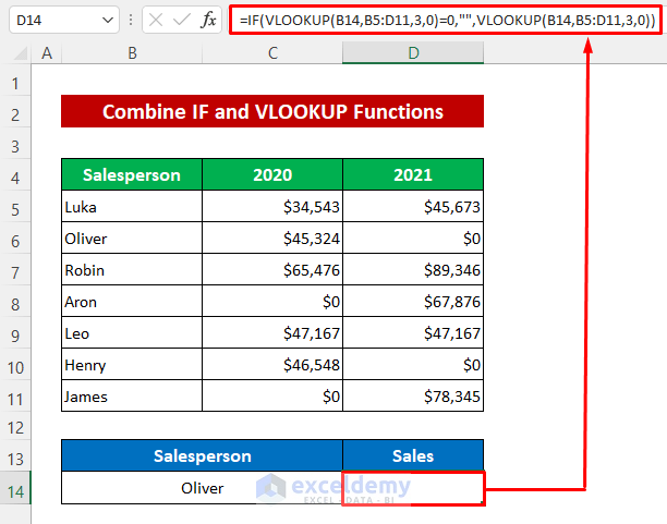
The following dataset contains some salespersons’ sales in two consecutive years. There are zero sales in some cells. We’ll use the IF and VLOOKUP functions in a formula to display blank cells in those cells instead.
![]()
Steps:
- Enter the following formula in Cell D14:
=IF(VLOOKUP(B14,B5:D11,3,0)=0,"",VLOOKUP(B14,B5:D11,3,0))- Press Enter.
The formula returns blank cells for the zero sales of Oliver.
Read More: How to Set Cell to Blank in Formula in Excel
Alternative Methods
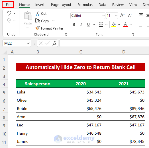
Method 1 – Automatically Hide Zero
Excel has an built in feature that will convert all the zeros to blank cells automatically.
Steps:
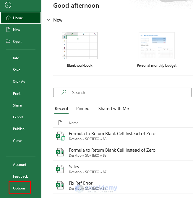
- Click File beside the Home tab.
- Click Options from the bottom section, and a dialog box will open up.
- Click the Advanced option.
- Select the sheet from the drop-down of Display options for this worksheet section.
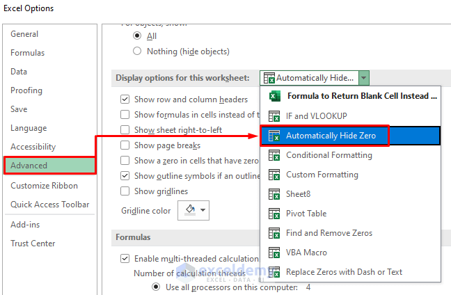
- Just unmark the Show a zero in cells that have zero value option.
- Click OK.
![]()
Blank cells will appear where all the zeros were before.
![]()
Read More: How to Make Empty Cells Blank in Excel
Method 2 – Using Conditional Formatting
Steps:
- Select the data range C5:D11.
- Click as follows: Home > Conditional Formatting > Highlight Cells Rules > Equal To.
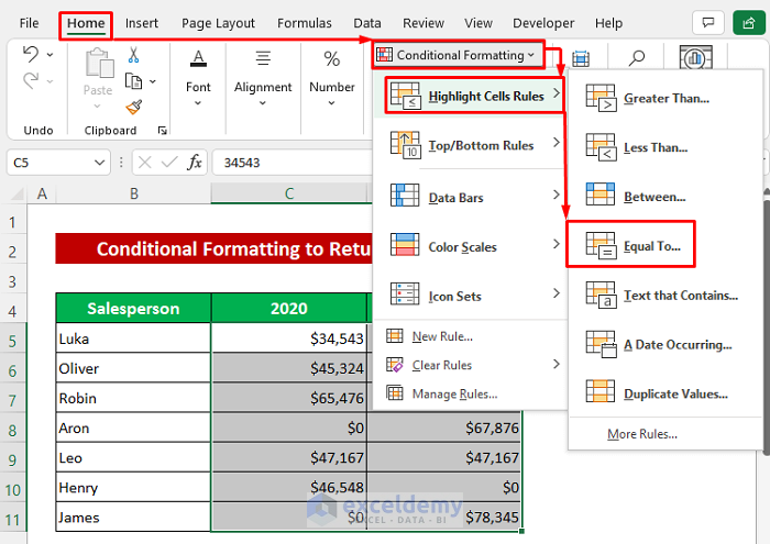
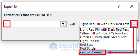
- Enter zero in the Format cells that are EQUAL TO box.
- Select Custom Format from the dropdown list.
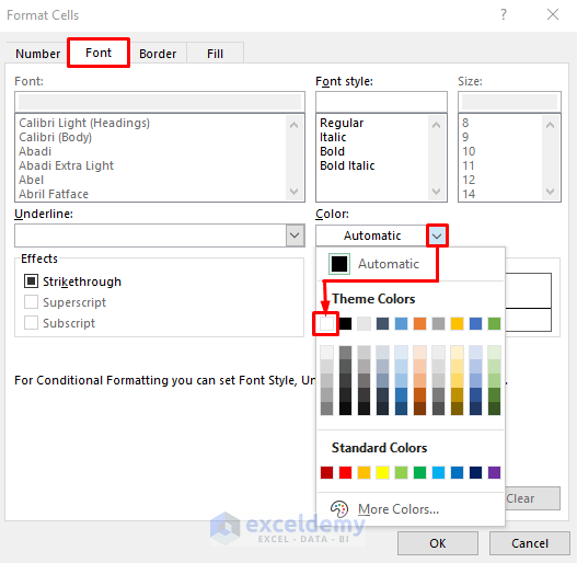
A Format Cells dialog box will open up.
- Click the Font option.
- Choose the white color from the Color section.
- Click OK.
- Alternatively, click Number > Custom and type three semicolons (;;;) in the Type box.
- Click OK and it will return to the previous dialog box.
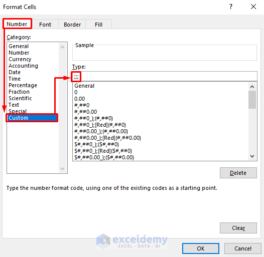
- Just click OK.
![]()
All the zero values are returned as blank cells.
![]()
Method 3 – Apply Custom Formatting
Steps:
- Select the data range.
- Right-click your mouse and select Format Cells from the Context menu.
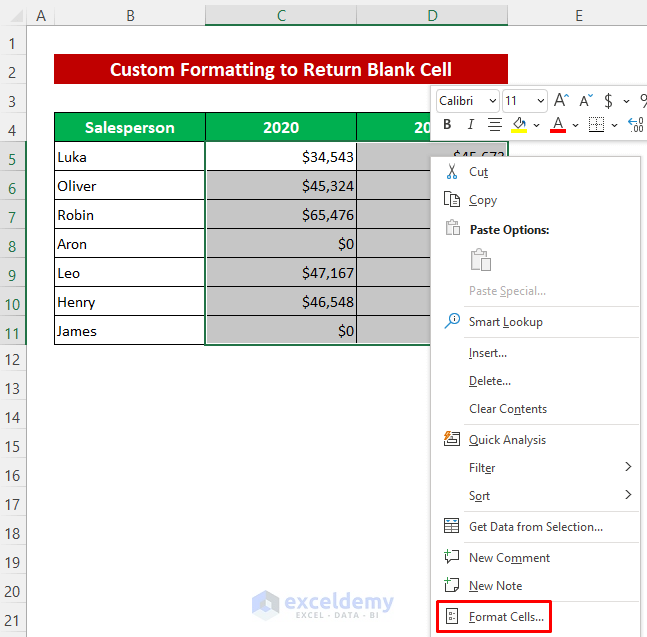
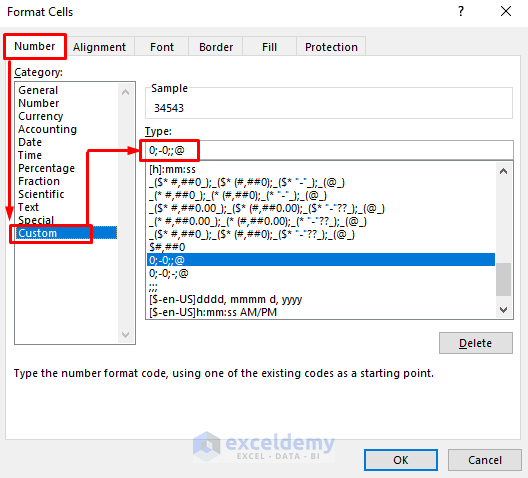
- From the Number section click Custom.
- Enter 0;-0;;@ in the Type box.
- Click OK.
Blank cells now appear where the zeros were.
![]()
Method 4 – Using Pivot Tables
Steps:
- Select the whole dataset.
- Click Insert > Pivot Table.
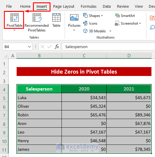
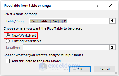
- Select your desired worksheet and click OK (here, New Worksheet).
- Select the data range from the Pivot Table.
- Click as follows: Home > Conditional Formatting > Highlight Cells Rules > Equal To.
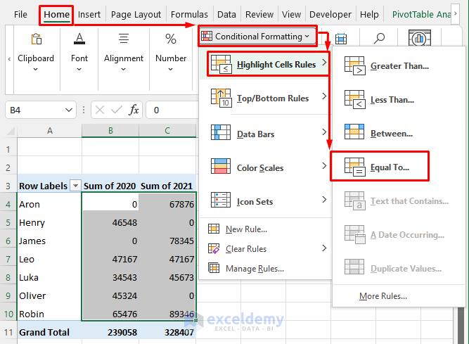
- Enter 0 (a zero) in the Format cells that are EQUAL TO box.
- Select Custom Format from the dropdown list.
A Format Cells dialog box will open up.
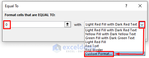
- From the Number section click Custom.
- Enter ;;; in the Type box and press OK.
![]()
And we are done.
![]()
Method 5 – Using Find and Replace
Steps:
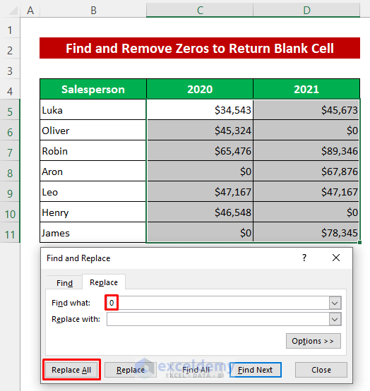
- Select the data range C5:D11.
- Press Ctrl+H to open the Find and Replace dialog box.
- Enter 0 (a zero) in the Find what box and keep the Replace with box empty.
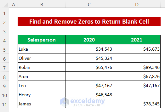
All the zeros are replaced with blank cells.
Replace Zeros with Dash or Specific Text
It’s as simple to replace zeros with a dash or specific text instead of blank cells.
Steps:
- Select the range of data.
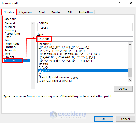
- Right-click your mouse and select Format Cells from the Context menu.
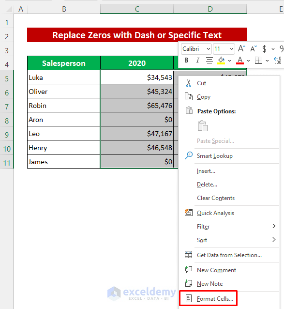
- From the Number section click Custom.
- Enter 0;-0;-;@ in the Type box to return a dash instead of zeros.
- Click OK.
The output will look like the image below.
![]()
- To return specific text, just replace the dash with whatever text you want within double quotes.
I typed NA.
- Then press OK.
![]()
The zeros in the cells now display ‘NA’.
![]()
Download Practice Workbook
Related Articles
- How to Find Blank Cells in Excel
- Null vs Blank in Excel
- How to Highlight Blank Cells in Excel
- How to Deal with Blank Cells That Are Not Really Blank in Excel
- Return Non Blank Cells from a Range in Excel
<< Go Back to Excel Cells | Learn Excel
Get FREE Advanced Excel Exercises with Solutions!
