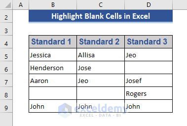
In this article, we will discuss 4 different methods to highlight blank cells in Excel. We’ll use the following dataset of the names of some students in different standards to illustrate our methods.
Method 1 – Highlight Blank Cells Using Conditional Formatting
We can use Conditional Formatting in different ways to highlight blank cells.
1.1 – Highlight All Blanks in a Range
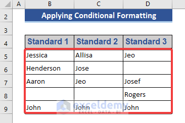
We can highlight blank cells with Conditional Formatting by customizing the fill color.
Steps:
- Select the range in which we will search for blanks and highlight them, by selecting the upper-left cell and pressing Ctrl+Shift+End.
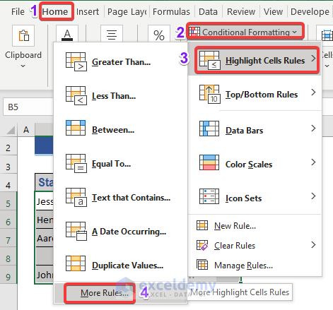
- Go to the Home tab.
- Click the Conditional Formatting option.
- Select More Rules from Highlight Cells Rules.
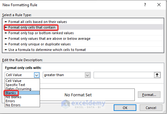
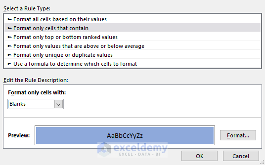
A new window named New Formatting Rule opens.
- Choose Format only cells that contain as Rule Type.
- Select Blanks as Format only cells with.
- Click on Format.
- Select the color for the Fill field.
- Click OK.
![]()
The Preview is displayed.
- Click OK.
![]()
The blank cells are highlighted in our chosen color.
1.2 – Highlight the Rows That Have Blank Cells (in a Specific Column)
Now we will highlight the rows that contain blank cells in a specific column using the ISBLANK function. If any cell of the specific column is blank, then that row will be highlighted.
Steps:
- Select the whole dataset by selecting the upper-left cell, and then pressing Ctrl+Shift+End.
![]()
- Go to the Home tab.
- Select New Rule from the Conditional Formatting command.
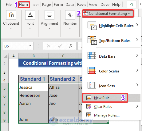
- Choose the option Use a formula to determine which cells to format from the Rule Type.
- Enter the following formula in the box indicated in the image below:
=ISBLANK($B5)- Click Format.
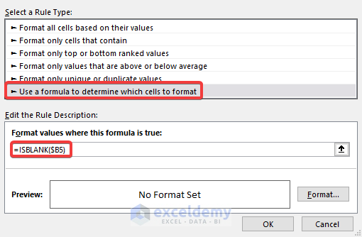
- Choose the desired color from the Fill tab.
- Click OK.
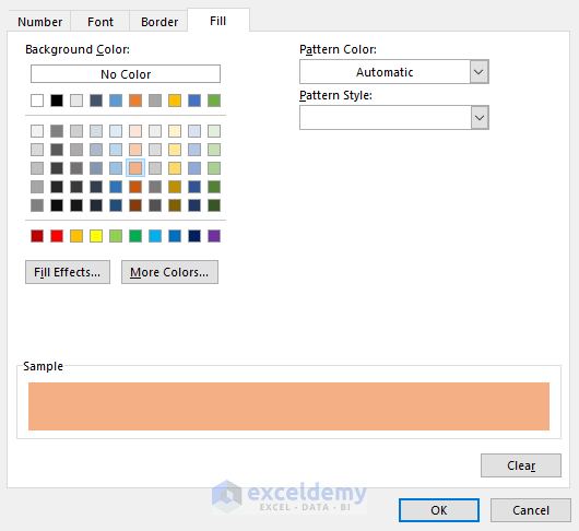
A Preview of the results is displayed.
![]()
- Click OK to return the final result.
![]()
The 8th row is highlighted as cell B8 is blank.
An Alternative to ISBLANK:
We can also use the LEN function to perform this operation. We’ll modify the formula and change the color format to accomplish this.
The formula is as follows:
=LEN($B5)=0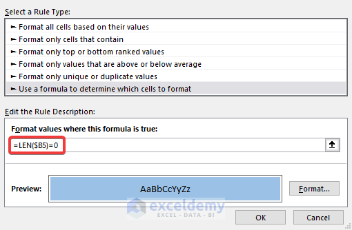
- After inputting the formula, click OK.
![]()
The LEN function delivers the same result.
1.3 – Highlight the Rows That Have Blank Cells (in Any Column)
Now we will use the COUNTBLANK function with conditional formatting to highlight the rows that contain blank cells in any column.
Steps:
- Enter the following formula as above:
=COUNTBLANK($B5:$D5)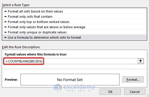
- Set the Format field and check the output in the Preview window.
![]()
- Click OK.
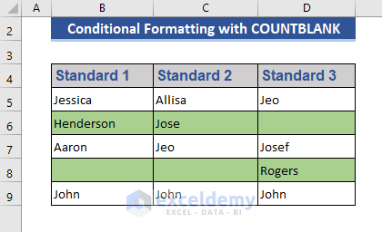
The rows which contain a blank cell in any column are highlighted.
Remove Conditional Formatting for Blank Cells:
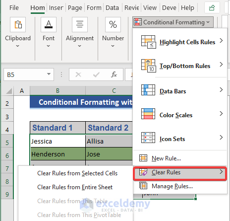
To remove the Conditional Formatting:
- Select Clear Rules from the Conditional Formatting drop-down.
- Clear rules from the Selected Cells or the Entire Sheet as required.
Read More: How to Find Blank Cells in Excel
Method 2 – Using Go To Special to Select and Highlight Blank Cells
Steps:
- Select the whole dataset.
![]()
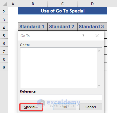
- Press F5 or Ctrl+G.
A new window named Go To will appear.
- Select Special.
The Go To Special window opens.
- Select Blanks.
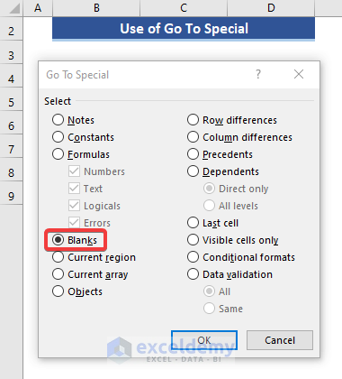
- Click OK.
![]()
The blank cells are marked.
Note:
- This method selects entirely blank cells. Cells containing spaces, empty strings, and non-printing characters are not considered as blanks.
- This is a one-time or static solution, meaning if we change the data, the changes will not be reflected.
Read More: How to Make Empty Cells Blank in Excel
Method 3 – Filter and Highlight Blank Cells in a Specific Column
The AutoFilter command can detect blank cells based on columns, but we’ll require a few more steps to highlight them afterwards.
Steps:
- Select the headings of all the columns in the dataset.
![]()
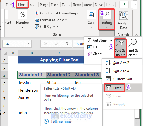
- Go to the Home tab.
- From the Editing command, click Sort & Filter.
- Select Filter.
- Or simply press Ctrl+Shift+L.
As indicated by the down-arrows next to the headings, the Filter option is activated.
![]()
- Click the drop-down and select Blanks.
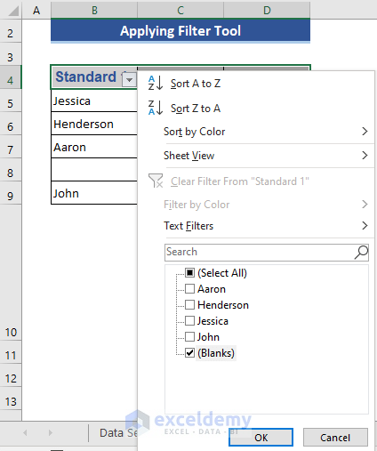
- Click OK.
![]()
Only the rows containing blank cells in Column B are showing. We can now highlight the blanks manually by filling in a color. Similarly, we can show and then highlight the blank cells in the other columns too.
Method 4 – Using VBA Macros to Highlight Blank Cells in Excel
For our last method, we will apply VBA codes to highlight blank cells in Excel, both for perfectly blank cells and for apparently blank cells that actually contain spaces or other invisible data.
4.1 – Highlighting Genuinely Blank Cells
Here is the dataset to which we will apply the VBA code:
![]()
Steps:
- Go to the Developer tab.
- Click on Macros.
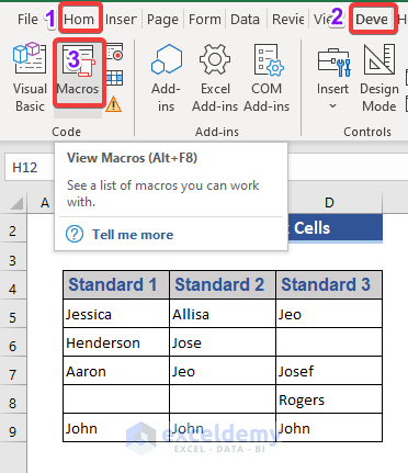
The Macro dialog box opens.
- Enter the Macro name as Hightlight_Blank.
- Click Create.
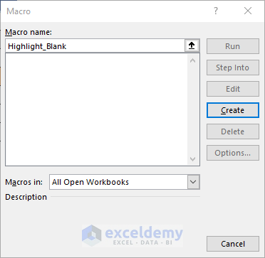
The command window of VBA opens.
- In it, enter the following VBA code:
Sub Highlight_Blank()
Dim Dataset As Range
Set Dataset = Range("B5:D9")
Dataset.SpecialCells(xlCellTypeBlanks).Interior.Color = RGB(255, 181, 106)
End Sub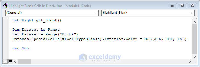
- Press F5 to run the code.
![]()
The blank cells are highlighted.
4.2 – Ignoring the Cells with Empty Strings
Steps:
- Modify the dataset by adding a space in a blank cell.
![]()
- Create a new Macro named Highlight_Empty_String.
- Click OK.
![]()
- Enter the following in the VBA command module:
Sub Highlight_Empty_String()
Dim Dataset As Range
Set Dataset = Range("B5:D9")
For Each cell In Dataset
If cell.Text = "" Then
cell.Interior.Color = RGB(255, 181, 110)
Else
cell.Interior.ColorIndex = xlNone
End If
Next
End Sub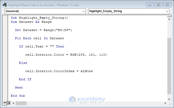
- Press F5 to run the code.
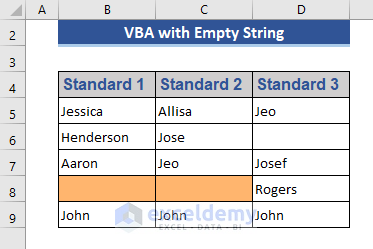
The cell containing the space is not highlighted, while the rest of the blank cells are.
Download Practice Workbook
Related Articles
- How to Deal with Blank Cells That Are Not Really Blank in Excel
- Return Non Blank Cells from a Range in Excel
- Null vs Blank in Excel
- How to Set Cell to Blank in Formula in Excel
- Formula to Return Blank Cell instead of Zero in Excel
<< Go Back to Excel Cells | Learn Excel
Get FREE Advanced Excel Exercises with Solutions!
