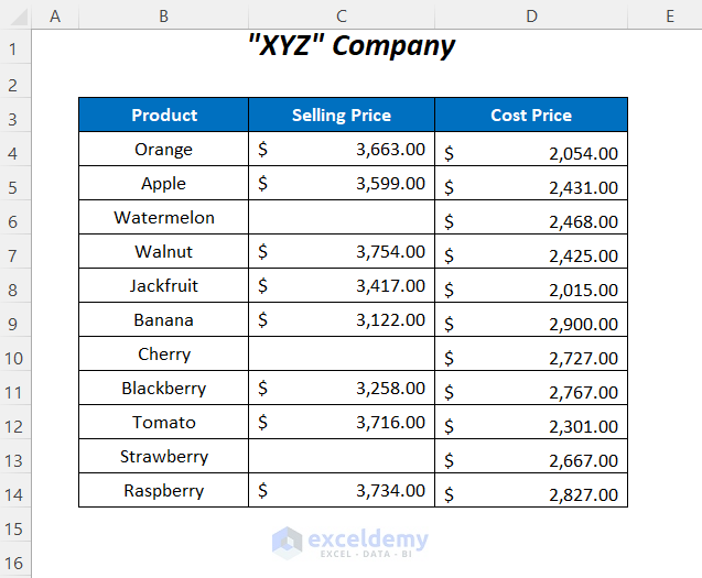
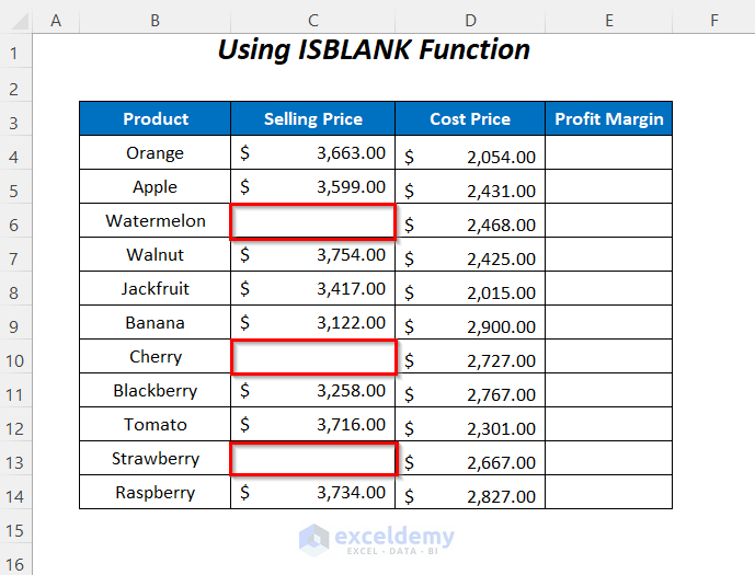
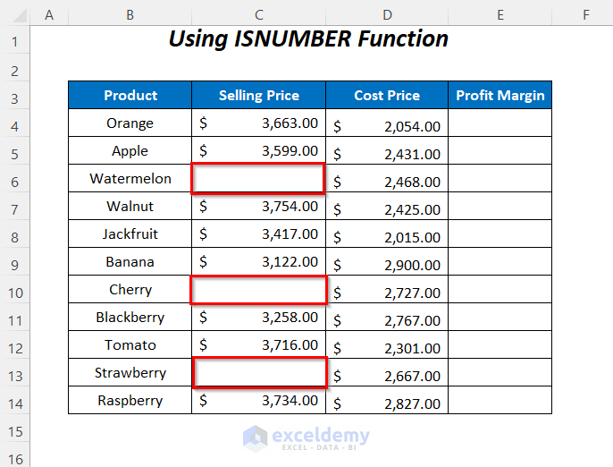
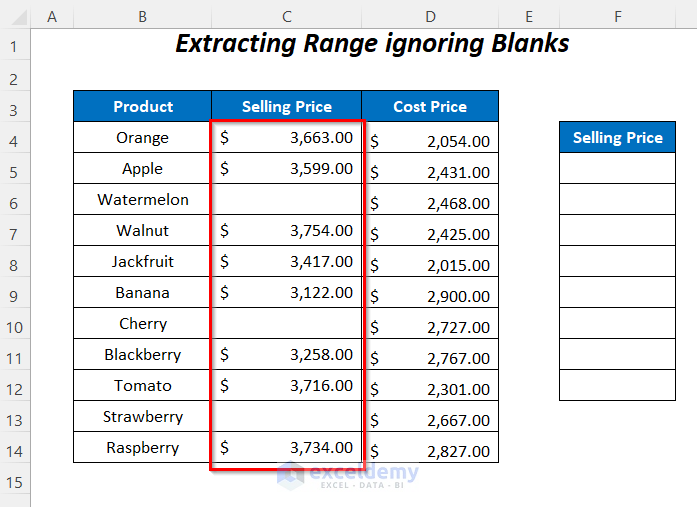
Consider the following dataset containing the Selling Price and Cost Price of some products of a company. We will use it to demonstrate how you can ignore the blank cells in the Selling Price column while performing calculations.
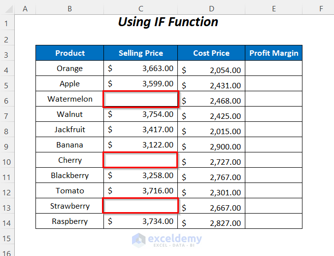
Method 1 – Ignore Blank Cells in a Range by Using the IF Function
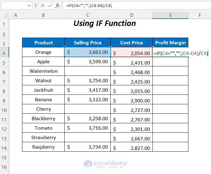
We will use the IF function to calculate the Profit Margin of the products, ignoring the blank cells in the Selling Price column since they’ll result in an error.
Here’s the general formula you could use to determine the Profit Margin for cell E4:
=(C4-D4)/C4 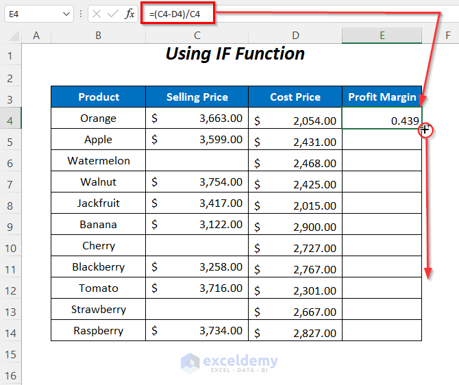
This results in the #DIV/0! error for the blank cells in the Selling Price column.
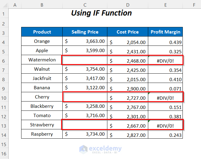
- To solve this problem, we will use the following formula to ignore the blank cells:
=IF(C4="","",(C4-D4)/C4)When C4 is blank it will return TRUE, then IF will return a blank otherwise we will get the Profit Margin.
- Press Enter and drag down the Fill Handle tool.
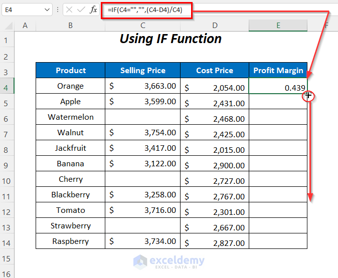
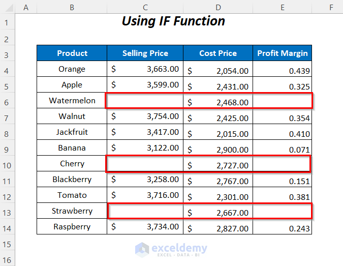
- You will get the profit margins of the products while ignoring the blank cells of the Selling Price column.
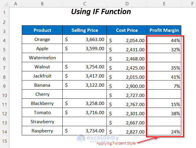
- Put the column values in the Percent Style.
Read More: How to Leave Cell Blank If There Is No Data in Excel
Method 2 – Using the ISBLANK Function to Ignore Blank Cells in a Range in Excel
In this section, we will be using the ISBLANK function to ignore the blank cells while calculating the Profit Margin of the Selling Price column.
Steps:
- Use the following formula in cell E4.
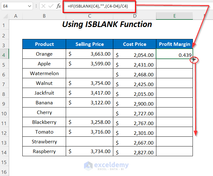
=IF(ISBLANK(C4),"",(C4-D4)/C4)- ISBLANK(C4) → returns TRUE for the blank cells and FALSE for the non-blank cells.
Output → FALSE
- (C4-D4)/C4 → gives the Profit Margin for Apple
Output → 0.439
- IF(ISBLANK(C4),””,(C4-D4)/C4) becomes
IF(FALSE,””,0.439) → returns the value 0.439 because the condition is giving FALSE
Output → 0.439

- Press Enter and drag down the Fill Handle tool.
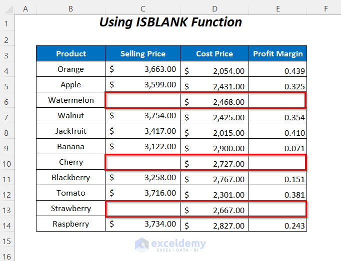
- You will get the Profit Margins for the products except for the products with blank selling prices.
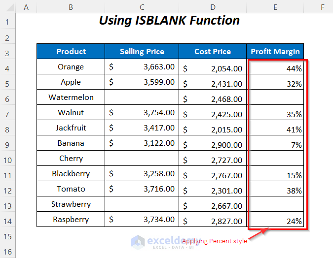
- Apply the Percent Style to the Profit Margin column.
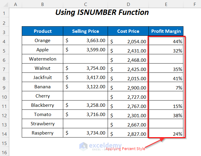
Method 3 – Using the ISNUMBER Function
You can use the ISNUMBER function to calculate the Profit Margins for the products in the same dataset.
Steps:
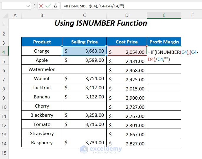
- Insert the following formula in cell E4.
=IF(ISNUMBER(C4),(C4-D4)/C4,"")- ISNUMBER(C4) → returns TRUE for the numbers otherwise FALSE (for checking texts you can use the ISTEXT function similarly)
Output → TRUE
- (C4-D4)/C4 → gives the Profit Margin for Apple
Output → 0.439
- IF(ISNUMBER(C4),(C4-D4)/C4,””) becomes
IF(TRUE, 0.439,””) → returns the value 0.439 because the condition is giving TRUE
Output → 0.439
- Press Enter and drag down the Fill Handle tool.
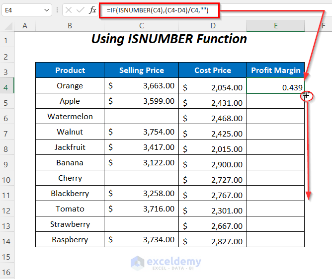
- You will get the Profit Margins for the products while ignoring the blank cells of the Selling Price column.
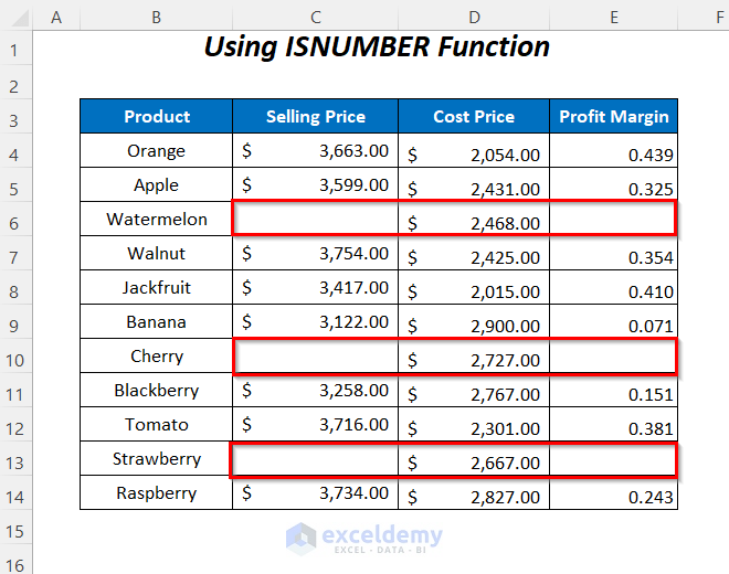
- After applying the Percent Style, we will get the following result.
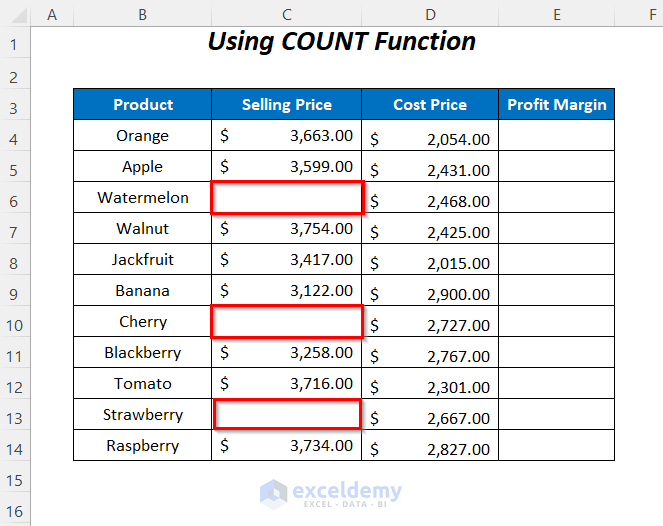
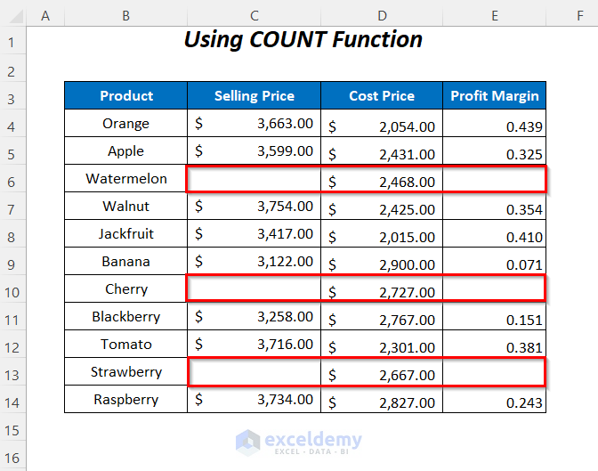
Method 4 – Using the COUNT Function to Ignore Blank Cells in a Range in Excel
We’ll use the same dataset as before.
Steps:
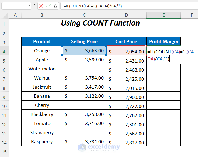
- Use the following formula in cell E4.
=IF(COUNT(C4)=1,(C4-D4)/C4,"")- COUNT(C4) → counts the number of cells containing numbers
Output → 1
- COUNT(C4)=1 becomes 1=1 and so returns TRUE.
- (C4-D4)/C4 → gives the Profit Margin for Apple
Output → 0.439
- IF(COUNT(C4)=1,(C4-D4)/C4,””) becomes
IF(TRUE,0.439,””) → returns the value 0.439 because the condition is giving TRUE
Output → 0.439
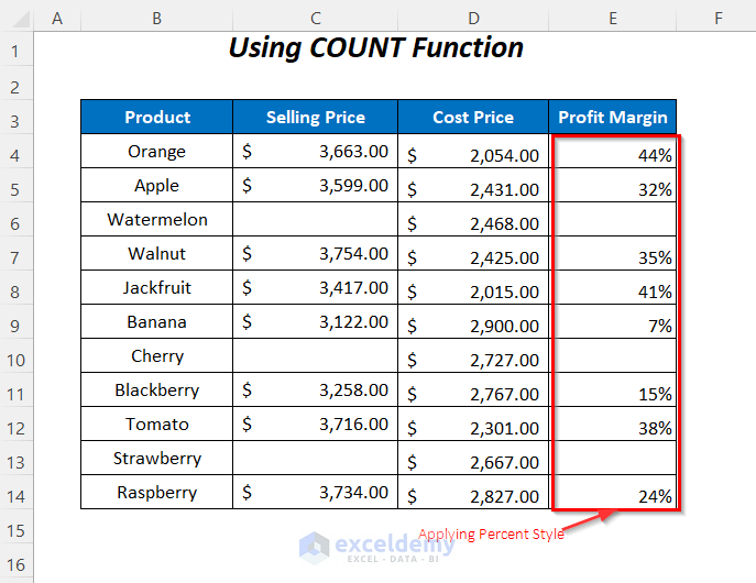
- Press Enter and drag down the Fill Handle tool.
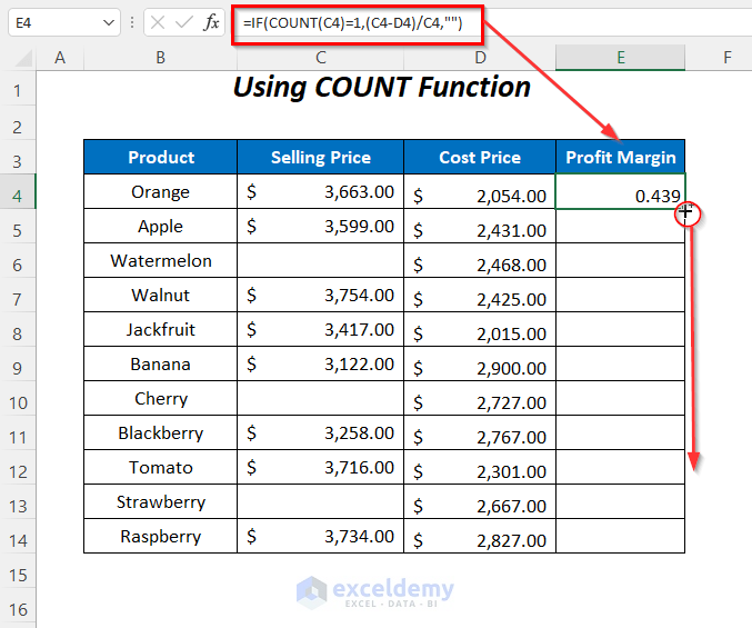
- You will get the Profit Margins for the products except for the products with blank selling prices.
- Apply the Percent Style to the Profit Margin column.
Method 5 – Ignore Blank Cells in a Range with the COUNTA Function
We’ll use the same dataset as before.
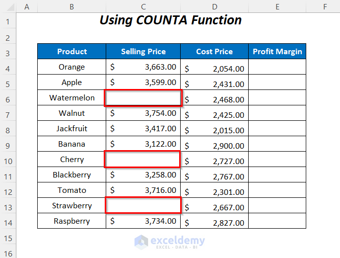
Steps:
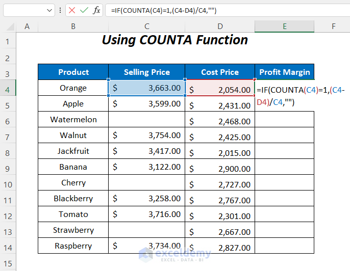
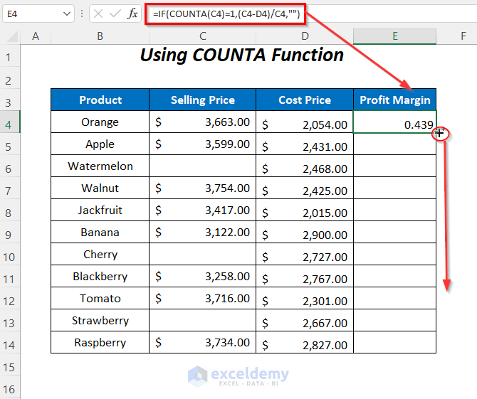
- Use the following formula in cell E4.
=IF(COUNTA(C4)=1,(C4-D4)/C4,"")- COUNTA(C4) → counts the number of cells containing numbers and texts
Output → 1
- COUNTA(C4)=1 → becomes 1=1 and so returns TRUE.
- (C4-D4)/C4 → gives the Profit Margin for Apple
Output → 0.439
- IF(COUNTA(C4)=1,(C4-D4)/C4,””) becomes
IF(TRUE,0.439,””) → returns the value 0.439 because the condition is giving TRUE
Output → 0.439
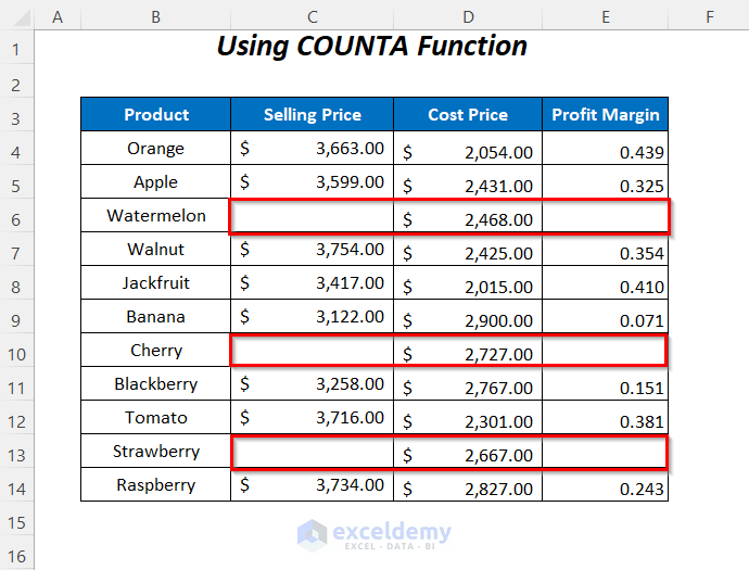
- Press Enter and drag down the Fill Handle tool.
- You will get the profit margins of the products ignoring the blank cells of the Selling Price column.
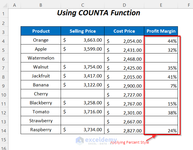
- After adding Percent Style, we are getting the following Profit Margins of the products.
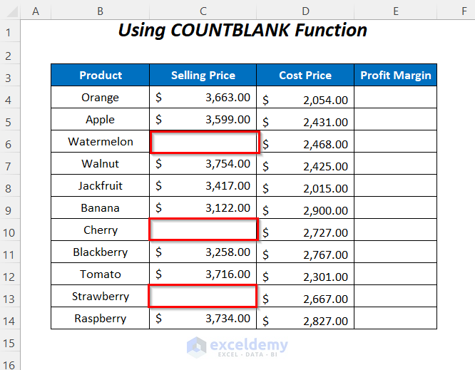
Method 6 – Using the COUNTBLANK Function to Ignore Blank Cells in a Range
We’ll use the same dataset as before.
Steps:
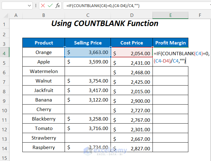
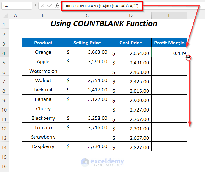
- Use the following formula in cell E4.
=IF(COUNTBLANK(C4)=0,(C4-D4)/C4,"")- COUNTBLANK(C4) → counts the number of blank cells
Output → 0
- COUNTBLANK(C4)=0 → becomes 0=0 and so returns TRUE.
- (C4-D4)/C4 → gives the Profit Margin for Apple
Output → 0.439
- IF(COUNTBLANK(C4)=0,(C4-D4)/C4,””) becomes
IF(TRUE,0.439,””) → returns the value 0.439 because the condition is giving TRUE
Output → 0.439
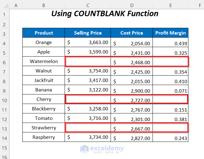
- Press Enter and drag down the Fill Handle tool.
- You will get the Profit Margins for the products except for the products with blank selling prices.
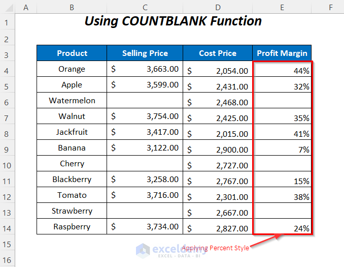
- Apply the Percent Style to the Profit Margin column.
Method 7 – Extracting a Range While Ignoring the Blank Cells
We will extract the values from the left Selling Price column to the right Selling Price column.
Steps:
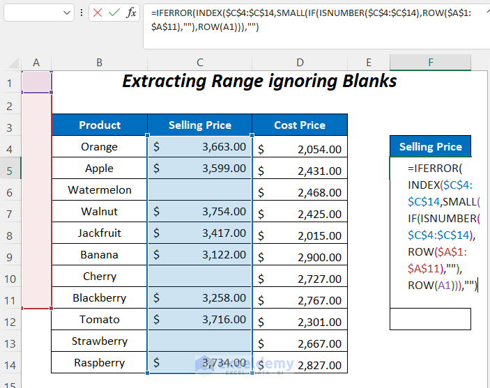
- Use the following formula in cell F5.
=IFERROR(INDEX($C$4:$C$14,SMALL(IF(ISNUMBER($C$4:$C$14),ROW($A$1:$A$11),""),ROW(A1))),"")ISNUMBER($C$4:$C$14)→ returns TRUE for the numbers otherwise FALSE
Output →{TRUE;TRUE;FALSE;TRUE;TRUE;TRUE;FALSE;TRUE;TRUE;FALSE;TRUE}
ROW($A$1:$A$11)→ returns the row numbers of this range
Output →{1;2;3;4;5;6;7;8;9;10;11}
ROW(A1)→ returns the row number of this cell
Output → 1
IF(ISNUMBER($C$4:$C$14),ROW($A$1:$A$11),"")becomes
IF({TRUE;TRUE;FALSE;TRUE;TRUE;TRUE;FALSE;TRUE;TRUE;FALSE;TRUE},{1;2;3;4;5;6;7;8;9;10;11},"")→ returns the row numbers for TRUE otherwise blank
Output →{1;2; “”;4;5;6; “”;8;9; “”}
SMALL(IF(ISNUMBER($C$4:$C$14),ROW($A$1:$A$11),""),ROW(A1)))becomes
SMALL({1;2; “”;4;5;6; “”;8;9; “”},1)→ returns the 1st smallest value of this range
Output → 1
INDEX($C$4:$C$14,SMALL(IF(ISNUMBER($C$4:$C$14),ROW($A$1:$A$11),""),ROW(A1)))becomes
INDEX($C$4:$C$14,1)→ returns the 1st value of this range
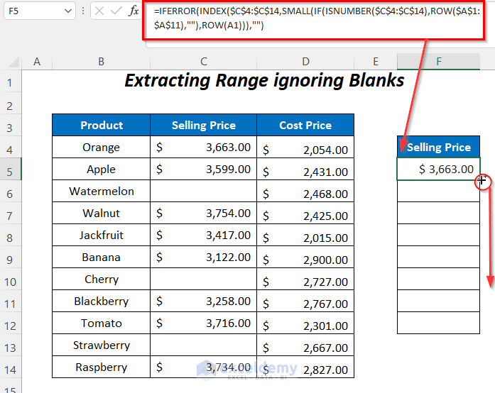
Output → 3663
IFERROR(INDEX($C$4:$C$14,SMALL(IF(ISNUMBER($C$4:$C$14),ROW($A$1:$A$11),""),ROW(A1))),"")becomes
IFERROR(3663,"")→ returns blank for any error
Output → 3663
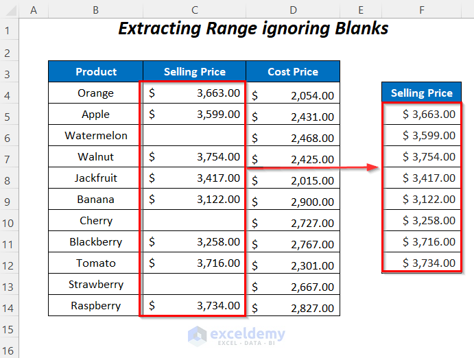
- Press Enter and drag down the Fill Handle tool.
- You will get the extracted values of the Selling Price column ignoring the blank cells.
Read More: How to Return Non Blank Cells from a Range in Excel
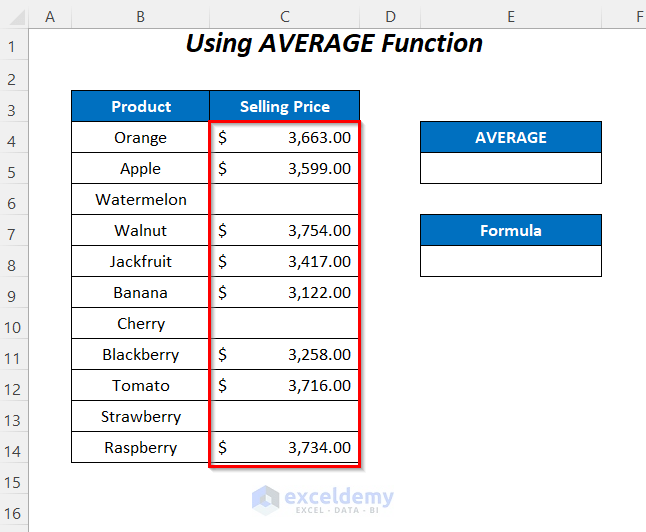
Method 8 – Ignore Blank Cells in a Range by Using the AVERAGE Function
Let’s get the average values while ignoring the blanks. We’ll insert a result cell, like below.
Steps:
- Enter the following formula in cell E5.
=AVERAGE(C4:C14)It will calculate the average of this range excluding the blank cells.
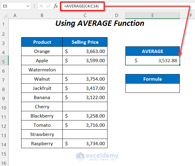
Now, we can check if the AVERAGE function is actually calculating the average excluding the blank cells.
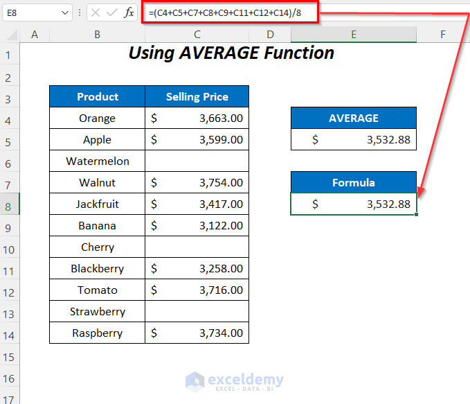
- Enter the following formula in cell E8.
=(C4+C5+C7+C8+C9+C11+C12+C14)/8Here, C4, C5, C7, C8, C9, C11, C12, C14 are the non-blank selling prices. We can see that the average values of the selling prices are the same.
Read More: How to Remove Blank Cells from a Range in Excel
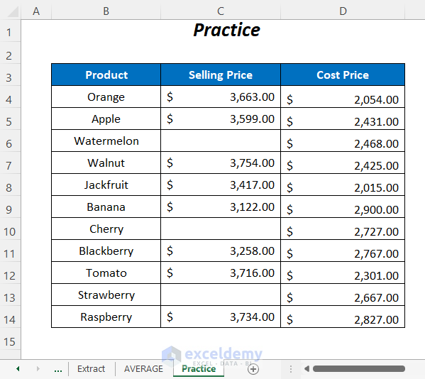
Practice Section
We have provided a Practice section like below in a sheet named Practice.
Download the Workbook
Related Articles
- How to Delete Blank Cells and Shift Data Up in Excel
- How to Delete Blank Cells and Shift Data Left in Excel
- How to Remove Unused Cells in Excel
- How to Remove Blank Cells in Excel
- How to Remove Blank Lines in Excel
<< Go Back to Excel Cells | Learn Excel
Get FREE Advanced Excel Exercises with Solutions!
