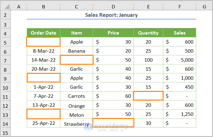
In the dataset below, the Sales Report for January is provided, and some cells are blank.
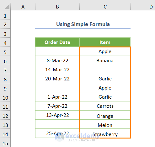
Method 1 – Using a Simple Formula
Steps:
- Select the C5:C14 cell range.
- Click on the New Rule option from the Conditional Formatting tool located in the Styles ribbon of the Home
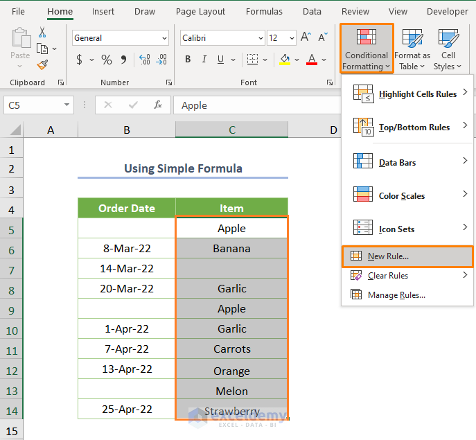
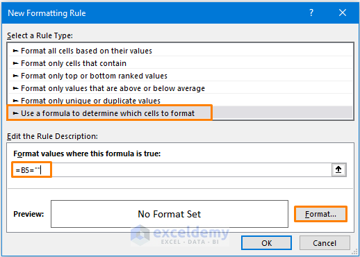
- In the dialog box, New Formatting Rule, choose the option Use a formula to determine which cells to format as a Rule Type.
- Insert the following formula in the Format values where this formula is true cell:
=B5=""
B5 is the first cell of the order date.
- Click on the Format option from the lower-right corner of the dialog box.
- Move the cursor over the Fill option and choose a highlighting color.
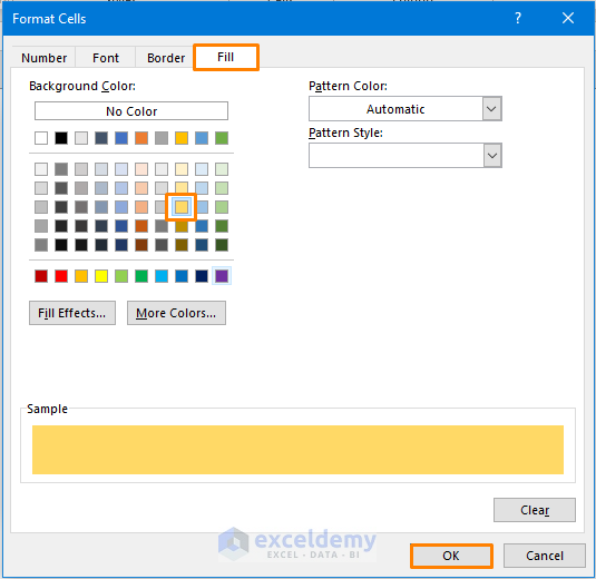
- Press OK to get the blank highlighted cells to have adjacent cells.
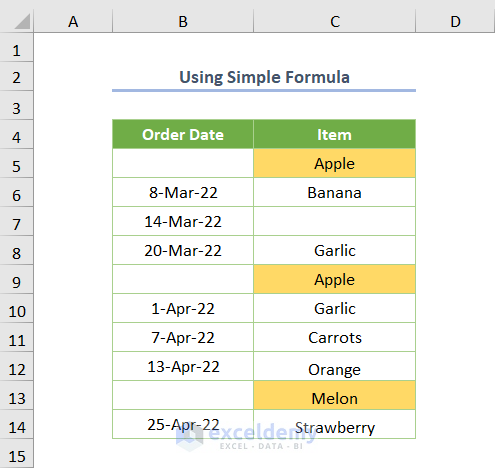
Conditional formatting highlights cells C5, C9, and C13 because cells B5, B9, and B13 are blank.
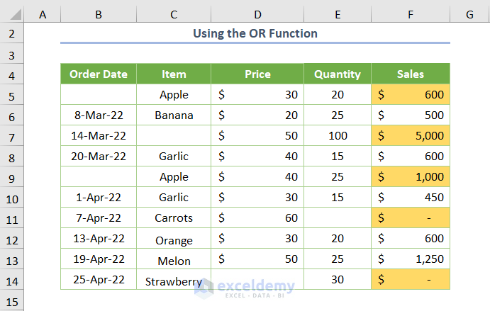
Method 2 – Using the OR Function If Another Cell Is Blank
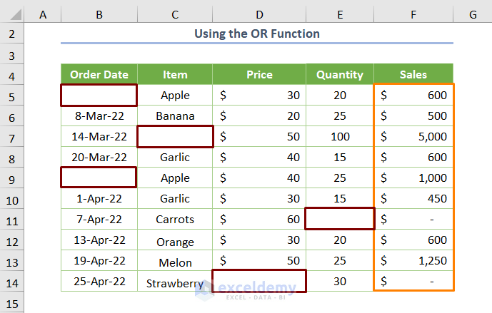
Highlight the specific cells from the F5:F14 cell range that have at least 1 blank cell of all fields using the OR function.
Stages:
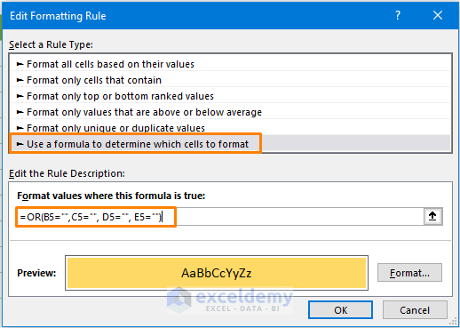
- Insert the following formula:
=OR(B5="",C5="", D5="", E5="")- B5, C5, D5, and E5 are the first cells of the date, item, price, and quantity fields, respectively.
The OR function shows correctly if at least one argument in any cell is blank. Conditional formatting highlights the cells that have at least 1 blank cell.
- You’ll get the following output.
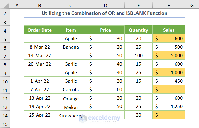
Method 3 – Utilizing the Combination of OR and ISBLANK Functions
Stages:
- Insert the following formula:
=OR(ISBLANK(B5),ISBLANK(C5),ISBLANK(D5),ISBLANK(E5))- The ISBLANK function returns true for a specific cell when the cell is blank. So, the function works as the same feature of double quotes (“”). The OR function returns true for all arguments.
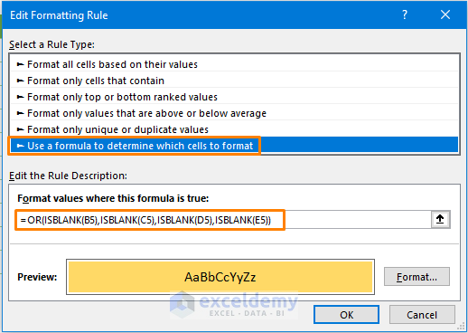
- Press OK to get the following highlighted cells.
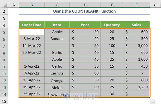
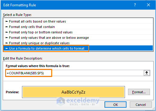
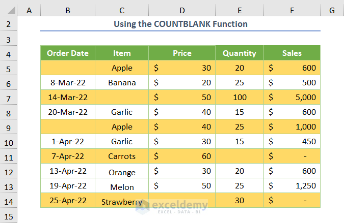
Method 4 – Using the COUNTBLANK Function If Another Cell Is Blank
Stages:
- Select the entire dataset.
- Insert the following formula:
=COUNTBLANK($B5:$F5)
F5 is the sales in a particular order date, which is found by multiplying the price and quantity.
- You’ll get the following highlighted rows.
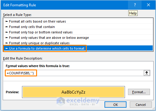
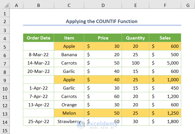
Method 5 – Applying the COUNTIF Function
Stages:
- Select the entire dataset.
- Enter the following formula:
=COUNTIF($B5,"")
- You’ll get the following output – the entire row is highlighted except the blank cell.
Download Practice Workbook
Related Articles
- How to Find & Count If a Cell Is Not Blank
- How to Calculate in Excel If Cells are Not Blank
- How to Return Value If Cell is Blank
- If a Cell Is Blank then Copy Another Cell in Excel
- Excel If Two Cells Are Blank Then Return Value
- How to Check If Cell Is Empty in Excel
- How to Check If Cell Is Empty Using Excel VBA
- Excel VBA: Check If Multiple Cells Are Empty
- If Cell is Blank Then Show 0 in Excel
<< Go Back to If Cell is Blank Then | Excel Cells | Learn Excel
Get FREE Advanced Excel Exercises with Solutions!
