How to Fill Blank Cells with Value Above in Excel (4 Easy Methods)

Let’s consider the following dataset. It contains the list of product IDs, sales dates, and sales numbers. Some of the cells have blank values, which we will fill in a few different ways.

Method 1 – Using Excel Go To Special Tool to Fill Blank Cells with the Value Above

Steps:

• Select the range of data where you want to fill the blank cells.

• Go to the Home tab and the Editing group, select the Find & Select drop-down menu and choose Go To Special.

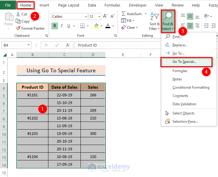
• A dialog box named Go To Special appears.
• Choose Blanks from the Go To Special box and click OK.

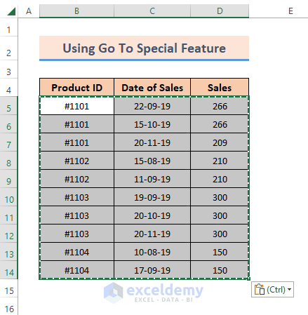
• This selects all blank cells.

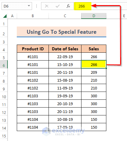
• Write the formula into the cell as “=D5“.

Here, D5 is the reference of the cell above, with whose value you want to fill in the blank cells.

• Press Ctrl + Enter, which fills the rest of the cells with a similar formula, using the previous cell’s reference.

Let’s convert the formulas into values.

• Select the entire dataset.
• Copy the entire dataset by pressing Ctrl + C.

• Right-click and select Paste Values (V).

• Finally, the result will look like the following picture.

The cells have been converted from having a formula (that you have applied) into a static value.

Method 2 – Applying the Find & Replace Command to Fill Blank Cells

Steps:

• Select the entire dataset.
• Go to the Home tab and the Editing group, select the Find & Select drop-down menu, and choose Find.

• A box will come up. Keep the Find what: box blank and click on Find All.

• Shift your cursor from the dialog box and place it on the worksheet, then press CTRL+A from the keyboard. This will select all the blanks.
• Click on Close to close the dialog box.

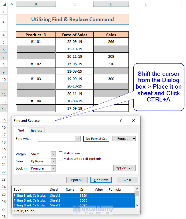
This will show the list of blanks in the selected range. For this dataset, the number of blanks found is 11.

• Press “=” from the keyboard, and an equal sign will automatically show up in the active cell.
• Write “D13” in the active cell.

• Press Ctrl+Enter.

Thus, you will find the result as shown.

Method 3 – Applying a Nested LOOKUP Formula in Excel to Fill Blank Cells

Steps:

• Select the whole data set.
• Choose Table from the Insert tab.

• The Create Table dialog box will open up and show the selected range of data.
• Mark My table has headers checkbox and click OK.

• Your dataset will look like a table with headers having arrow icons as shown below.

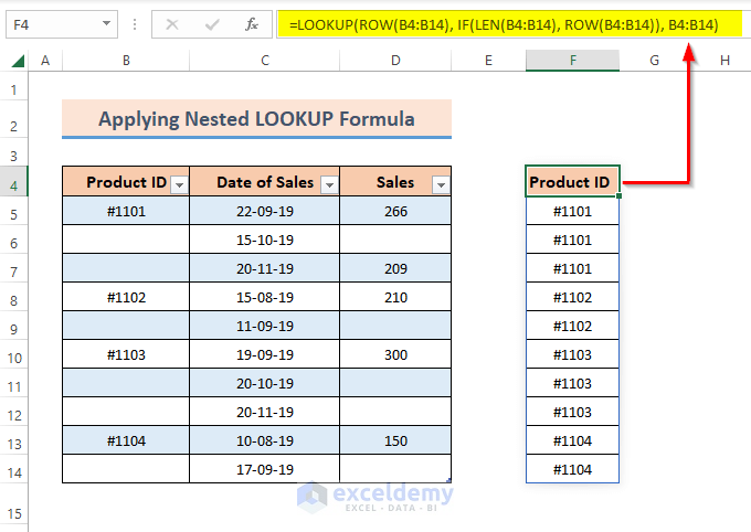
• Select a random column F and copy the following formula:

• The result will show the data of column B along with filling up the blanks with a value above that cell.

• Repeat the process for column C using the following formula:

• The values of Dates of Sales are different from the original dataset because the Number Format is General by default.

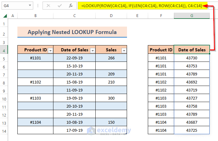
• Change the format by selecting Short Date instead of General.

Follow the picture to find where to change.

• Copy this formula into column H:

• This will give the following result:

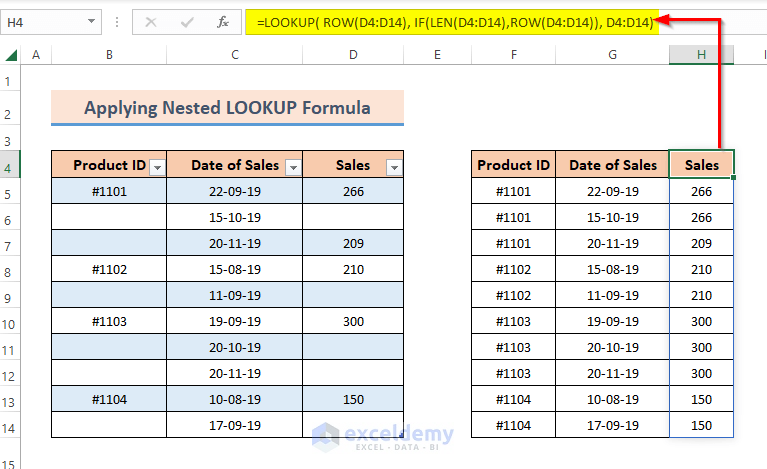
This method helps to have the original dataset and forms a new table to get the desired result.

Method 4 – Using Excel VBA to Fill Blank Cells with a Value Above

Steps:

• Select the dataset and right-click on the name of the sheet.
• Click on View Code from the Context menu.

• The VBA window will open showing the General Window on it.
• Copy the following code into it:

Code:

Sub FillCellFromAbove()
For Each cell In Selection
    If cell.Value = "" Then
        cell.Value = cell.Offset(-1, 0).Value
    End If
Next cell
End Sub

• Press F5 from the keyboard to run the code or click on the green arrow in the ribbon.

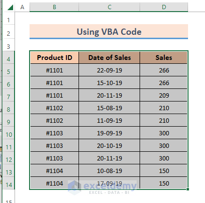
• The code will run, and you can see the result in the worksheet.

Download Practice Workbook

You can download the workbook from here.

Related Readings

• How to Fill Blank Cells with Value Below in Excel
• How to Fill Blank Cells with 0 in Excel
• Fill Blank Cells with Dash in Excel
• How to Fill Blank Cells with Color in Excel
• How to Fill Blank Cells with Value from Left in Excel

<< Go Back to Fill Blank Cells | Excel Cells | Learn Excel