Method 1 – Applying Go To Special Feature and a Formula
Steps:
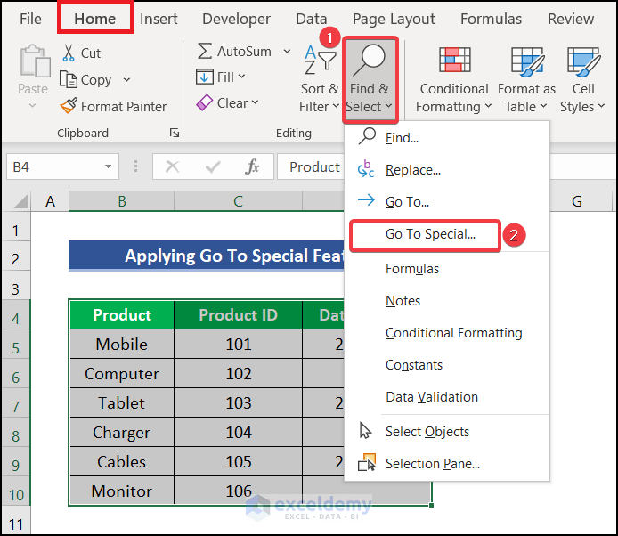
- Select the entire dataset (B4:D10) and go to Find & Select under Home tab.
- Click on Go to Special.
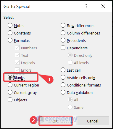
- A dialog box named Go To Special will appear. Check the Blanks option and hit OK.
- The empty cells will be highlighted.
![]()
- Press the Equal to (=) button from the keyboard in the active cells and select the last value you entered.
- Press CTRL + ENTER for the other empty cells. It will be filled with the last value of previous cells.
![]()
- Your empty cells will be filled with the last value above them.
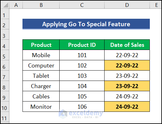
Note: You can format your empty cells according to your preference.
Method 2 – Employing Find and Replace Feature
Steps:
- Go to the Home tab >> under the Editing group, pick Find & Select >> select Find.
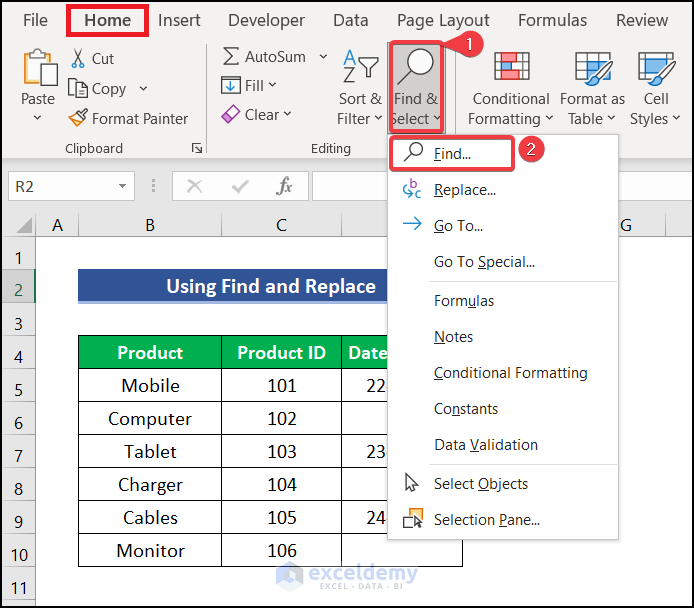
Note: You can also open the Find command by using Ctrl + H from the keyboard.
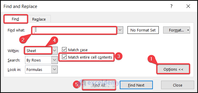
- The Find and Replace dialog wizard will pop out.
- Under the Find tab, select Options, keep the Find what box blank, check Match entire cell contents, for Within set Sheet.
- Press Find All.
- It will show you all the empty cells in your dataset. You can select all of them with CTRL + A.
- Hit the Close option.
![]()
- All the empty cells will be highlighted.
- Insert (=) in the active cell D10 and click on the last value you entered in cell D9.
- Press CTRL + ENTER for other empty cells to be filled with the last value.
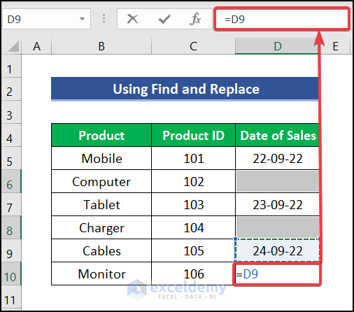
- Here are the results.
![]()
Method 3 – Using a Nested LOOKUP Formula
Steps:
- Select the entire data range, go to the Insert tab, and choose the Table option.
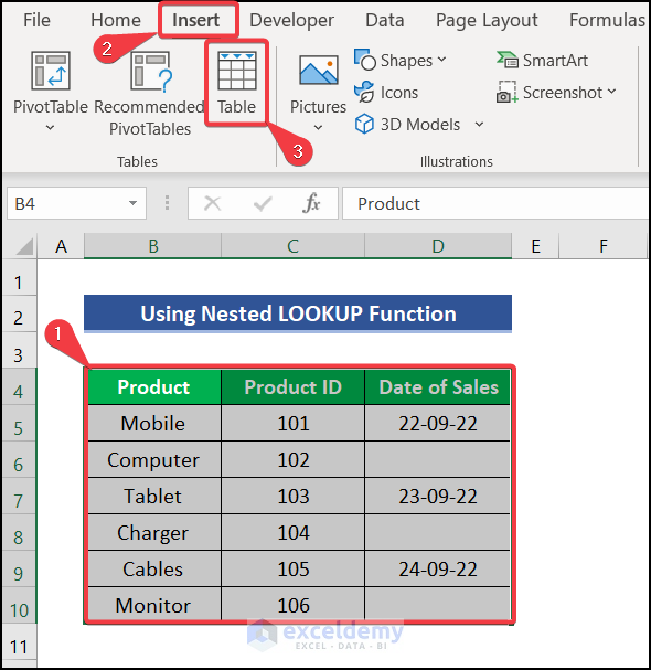
- A Create Table dialog box will pop out. Check My table has headers and press OK.
![]()
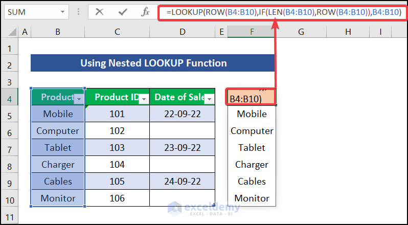
- Go to the F4 cell and insert this formula.
=LOOKUP(ROW(B4:B10),IF(LEN(B4:B10),ROW(B4:B10)),B4:B10)Formula Breakdown:
=LOOKUP(lookup_value, lookup_vector, [result_vector])
- Lookup_value takes the data we want to find. Since we have multiple rows in our data set the ROW function is working here which takes the range of the column. In our dataset, the ROW function will take the B4:B10 column value.
- lookup_vector is using the IF function nested with the LEN function and the ROW function. Both take the range of columns to create a vector form. The LEN function counts the character length, and the ROW function returns the column value. The IF function will give the output (4,5,6,7,8,9,10) which will be row numbers.
- result_vector is the result value taken in the form of a vector to get the desired result. It returns the result of the Products column.
- Go to the G4 cell and use a similar formula.
=LOOKUP(ROW(C4:C10),IF(LEN(C4:C10),ROW(C4:C10)),C4:C10)- This will create a new column of Product ID.
![]()
- Go to cell H4 and enter the same formula changing the reference column. It will create the Date of Sales column where the empty cells are filled with the last value. The formula is:
=LOOKUP(ROW(D4:D10),IF(LEN(D4:D10),ROW(D4:D10)),D4:D10)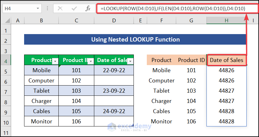
- Go to the Home tab and select Short Date in the Number format selector.
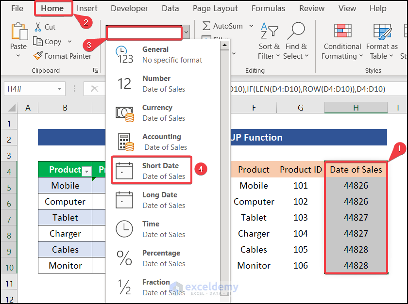
- The empty cells are filled with the last value.
![]()
Method 4 – Using VBA Macro to Fill Empty Cells with the Last Value
Steps:
- Select the entire range of your dataset and go to the Developer tab, then select Visual Basic.
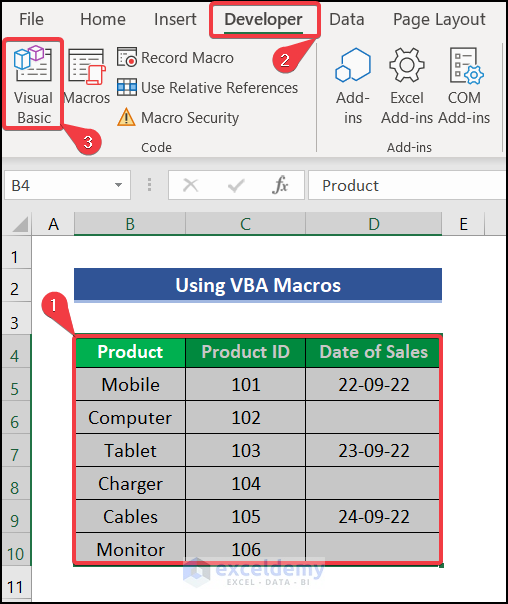
- A new dialog box will appear. Choose the Insert tab and go to Module.
![]()
- Insert this code in the new module.
Sub Fill Cell From Last Value ()
For Each cell In Selection
 If Cell. Value = "" Then
 Cell. Value = Cell. Offset(-1, 0).Value
    End If
Next cell
End Sub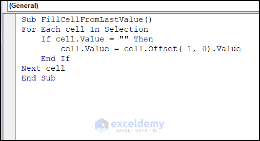
- Run the code.
![]()
How to Fill Blank Cells with 0 in Excel
Steps:
- Select the entire dataset range and go to the Home tab.
- Choose the Find & Select command and click Replace.
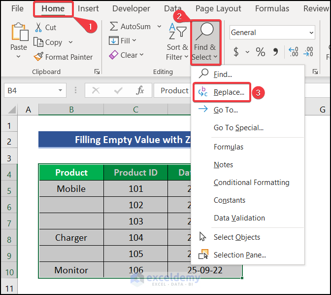
- A dialog window for Find and Replace will open. Go to the Replace tab.
- Press Options.
- Check Match entire cells content.
- Keep the Find what box blank.
- Select Sheet in the Within box.
- Put a 0 in the Replace with box.
- Click on Replace All.
![]()
- The empty cells will be replaced by 0.
How to Fill Empty Cells with Default Value in Excel
Steps:
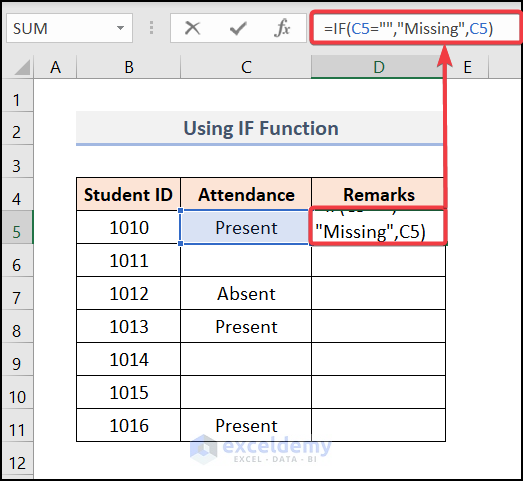
- Select the cell D5 and insert this formula:
=IF(C5="","Missing",C5)The syntax =IF(C5=””,”Missing”,C5) will check if cell C5 contains a blank cell. If the logic is TRUE then it will return Missing. It will return the same value in C5.
- Press ENTER.
- Drag down the Fill Handle tool for the other cells.
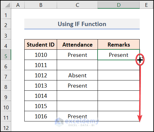
- Here’s the result.
![]()
Download the Practice Workbook
Related Articles
<< Go Back to Fill Blank Cells | Excel Cells | Learn Excel
Get FREE Advanced Excel Exercises with Solutions!
