Example 1 – Use the Intersection Command and a Function Button in Excel
Steps:
- Press F9.
- Enter the first level of rows, here C5:E7.
- Enter a space after it.
- Select B6:E6.
- Press Enter.
- The intersecting range between the two ranges is displayed in C14.
Example 2 – Using Named Ranges to Determine Intersecting Ranges in Excel
- Select C5:C7 and go to the Name Box.
- Enter Institute_1.
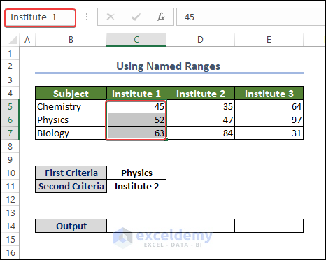
- Repeat this process for D5:D7 and E5:E7.
- Name B6:E6 as Physics.
You can see the named ranges in Name Manage.
- Select C14 and enter the following formula:
=Institute_1:Institute_2 Physics- Press F9.
The intersecting range is displayed between the two ranges in C14.
Example 3 – Using the Intersection Command to Sum Values
Steps:
- Select a cell and enter the following formula:
=SUM(C5:E7 B6:E6)
- Press F9.
You can see the summation of the intersecting ranges C6:E6 in C10.
Example 4 – Using the Intersection Command to Get the Maximum and Minimum of the Intersecting Cells
Steps:
- Select D10, and enter the following formula:
=MAX(C5:E7 B6:E6)
- Press F9.
You can see that the maximum value in the intersection values.
Repeat the process and get the minimum value of the intersected cells.
- Enter the following formula in C12 and press F9.
=MIN(C5:E7 B6:E6)
You can see the minimum cell value in the intersected cells.
Example 5 – Implementing a VBA Macro to Extract Intersecting Values
To display the developer tab, click here.
Steps:
- Open the visual basic in the Developer tab.
- Go to Insert > Module.
- Enter the code.
Sub ExtractIntersect()
    Dim colRange As Range
    Dim intersectRange As Range
    Dim intersectingCells As Range
    Dim cell As Range
    Dim intersectingValues() As Variant
    Dim i As Integer
    Set colRange = Application.InputBox("Select the column to check for intersecting values", "Select Column", Type:=8)
    Set intersectRange = Application.InputBox("Select the range to check for intersecting values", "Select Range", Type:=8)
    Set intersectingCells = Application.Intersect(colRange, intersectRange)
    ReDim intersectingValues(1 To intersectingCells.Cells.Count)
    i = 0
    For Each cell In intersectingCells
        i = i + 1
        intersectingValues(i) = cell.Value
    Next cell
    If i > 0 Then
        MsgBox "The following values are intersecting between the selected column and range:" & vbCrLf & Join(intersectingValues, vbCrLf)
    Else
        MsgBox "There are no intersecting values between the selected column and range."
    End If
End Sub
VBA Code Breakdown
Sub ExtractIntersect()
    Dim colRange As Range
    Dim intersectRange As Range
    Dim intersectingCells As Range
    Dim cell As Range
    Dim intersectingValues() As Variant
Dim i As Integer- declares several variables: it sets up a Range variable for the column to check (colRange), a Range variable for the range to check (intersectRange), a Range variable for the cells that intersect (intersectingCells), a Range variable for each individual cell (cell), an array variable to store the intersecting values (intersectingValues), and a counter variable (i).
Set colRange = Application.InputBox("Select the column to check for intersecting values", "Select Column", Type:=8)
Set intersectRange = Application.InputBox("Select the range to check for intersecting values", "Select Range", Type:=8)- prompts the user to select the column and the range to check using an input box. The Type:=8 parameter specifies that the user must select a range of cells.
Set intersectingCells = Application.Intersect(colRange, intersectRange)- checks for the intersection between the two ranges selected by the user and stores the result in the intersectingCells variable.
ReDim intersectingValues(1 To intersectingCells.Cells.Count)
i = 0
For Each cell In intersectingCells
    i = i + 1
    intersectingValues(i) = cell.Value
Next cell- loops through each cell in the intersectingCells range and adds the cell value to the intersectingValues array. The ReDim statement resizes the array to accommodate the number of intersecting cells.
If i > 0 Then
    MsgBox "The following values are intersecting between the selected column and range:" & vbCrLf & Join(intersectingValues, vbCrLf)
Else
    MsgBox "There are no intersecting values between the selected column and range."
End If- displays a message box that lists the intersecting values between the selected column and range, separated by a new line. If there are no intersecting values, it displays a message indicating so.
- Click Run.
- You will see an inputbox asking for the first range of cells: here D5:D7.
- There will be another inputbox asking for the second range of cells: B6:E6.
- A message box displays the intersected value.
Frequently Asked Question
- What is Union Operator in Excel?
The union operator is used to combine two or more ranges into a single range. The union operator is represented by a comma (,) between two or more range references.
To combine A1:A5 with C1:C5, enter it as “A1:A5, C1:C5” (without quotes) using the union operator.
Here’s an example of how to use the union operator in a formula:
=SUM(A1:A5,C1:C5)- How do I find the intersection of two columns in Excel?
Normally, there is no intersection between two columns, but you can find an intersection value : the same value in both columns:
- To find the intersection between Sales of Product A and Sales of Product B, enter the following formula in G5,
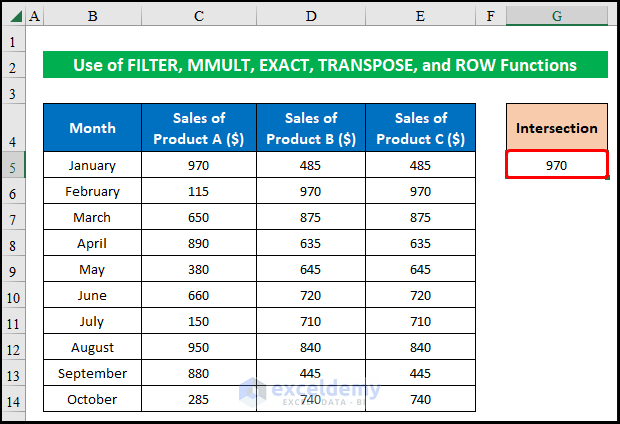
=FILTER($C$5:$C$14,MMULT(EXACT(C5:C14,TRANSPOSE(D5:D14))*1,ROW(C5:C14)^0))
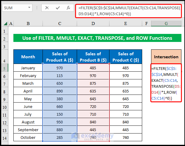
- Press Enter to see the intersection value between the two column values.
Things to Remember
- The ranges must have the same number of rows and columns for the intersection operation to work.
- If there is no intersection between the specified ranges, the result will be an empty cell or range.
- You can use the intersection operator with more than two ranges.
- The intersection operator is case-insensitive, so you can use upper- or lowercase letters when specifying ranges.
Download Practice Workbook
Download the Excel workbook.
Related Articles
<< Go Back to Excel Operators | Excel Formulas | Learn Excel
Get FREE Advanced Excel Exercises with Solutions!
