How to Perform an Intersection of Two Data Sets in Excel (4 Methods)

Dataset Overview

Let’s dive into the methods for finding the intersection of two data sets in Excel. We’ll use a sample dataset representing Month-wise Sales for Sales Reps. Here are the four methods:

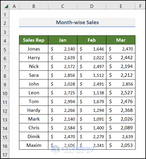
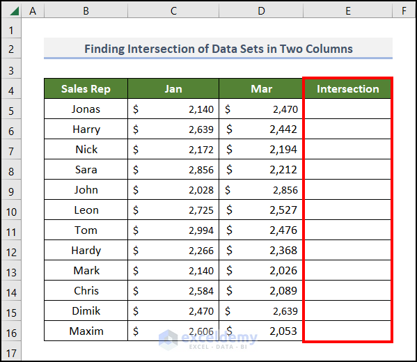
Method 1 – Finding Intersection of Data Sets in Two Columns

Steps

• Create a new column labeled Intersection under Column E.

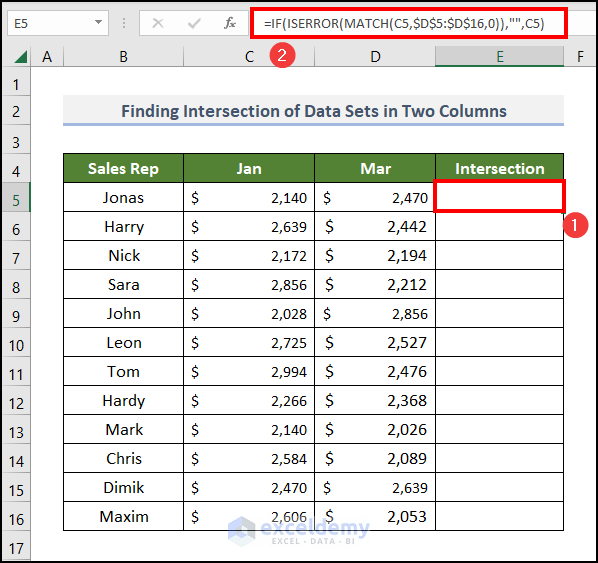
• In cell E5, use the following formula:

• Press ENTER.

• Double-click the Fill Handle tool (the plus sign at the right-bottom corner of cell E5) to copy the formula to lower cells.

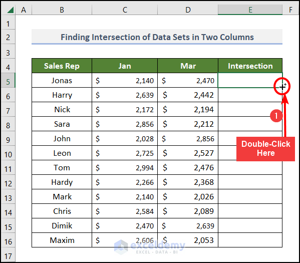
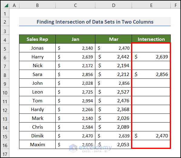
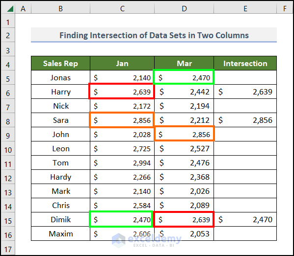
• The Intersection column will contain values available in both columns C and D.

Read More: Intersection of Two Columns in Excel

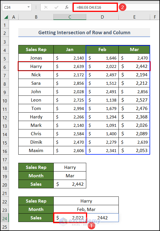
Method 2 – Getting Intersection of Row and Column in Excel

Steps

• In cells C18 and C19, provide a random name for the Sales Rep and Month.

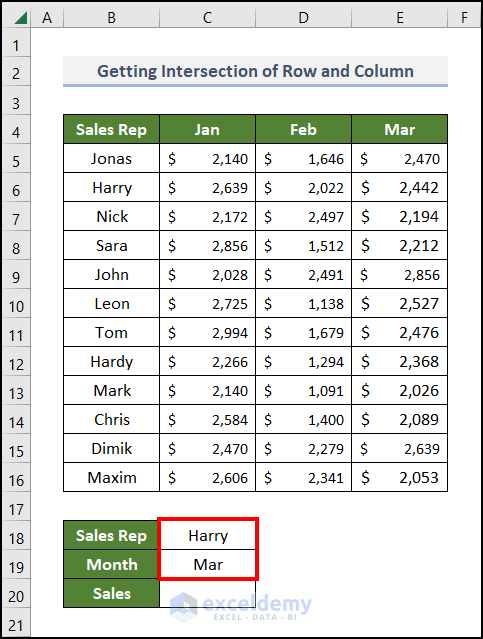
• To find Harry’s sales amount in March, select cell C20 and paste the formula:

• • This formula calculates the intersection of row 6 (Harry) and column E (March).

• Press ENTER.

• Similarly, you can find sales amounts for the same Sales Rep in February and March using the formula:

• • Adjust the row and column references as needed.

Read More: How to Use Intersection Operator in Excel

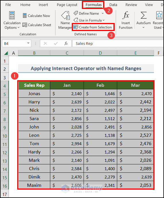
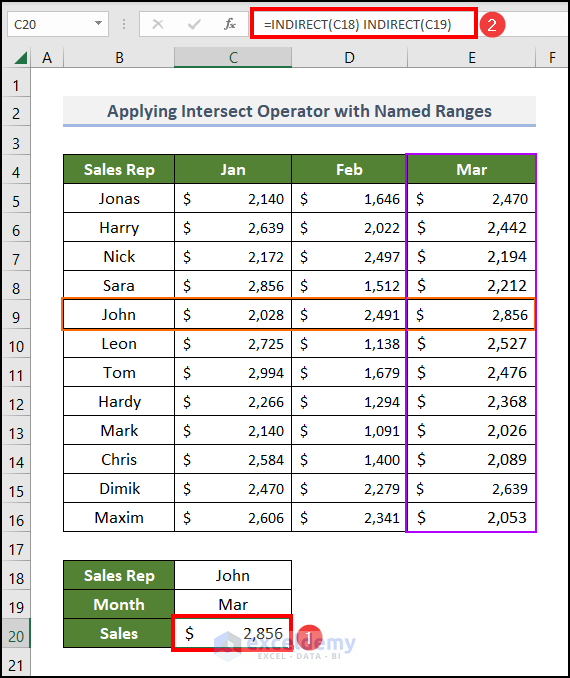
Method 3 – Applying Intersect Operator with Named Ranges

Steps

• Highlight the entire dataset in the B4:E16 range.
• Navigate to the Formulas tab.
• Click on Create from Selection.

• In the Create Names from Selection dialog box, check the boxes for Top row and Left column, then click OK.

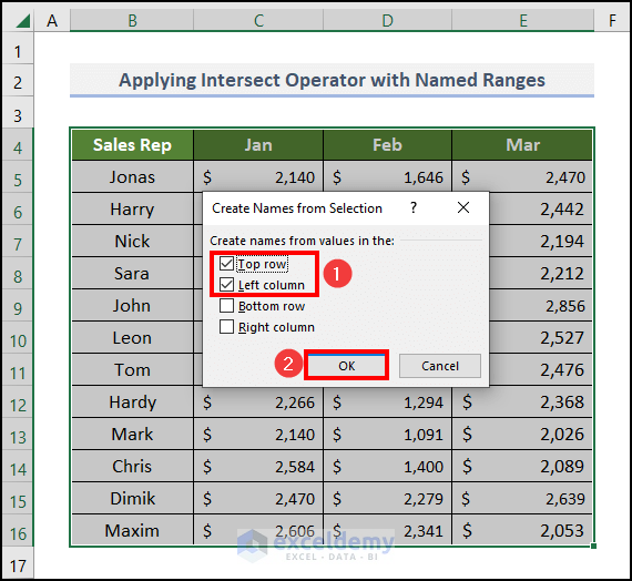
• Now, the columns and rows have their respective names.
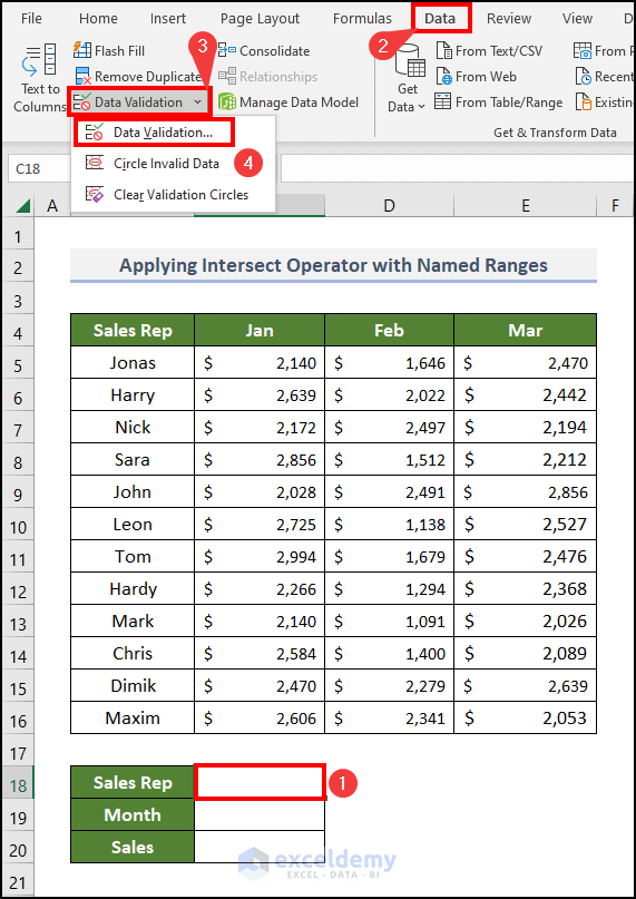
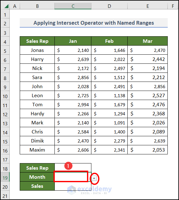
• Enlist the names of Sales Reps and Months in cells C18 and C19, respectively, using Data Validation:
  • Go to cell C18.
  • Proceed to the Data tab.
  • Click on the Data Validation drop-down on the Data Tools group.
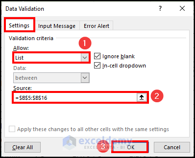
  • Select the Data Validation option from the list.

• In the Allow box, select List.
• In the Source box, reference the B5:B16 range.
• Click OK.

• Repeat the same process for cell C19. Use the down arrow beside these two cells when you click on the cells.

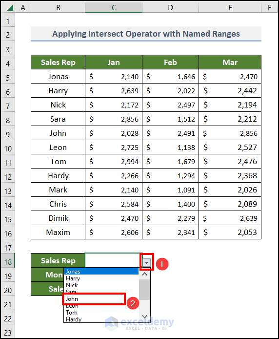
• lick on the arrow beside cell C18, and from the list, select John.

• Choose Mar in cell C19.

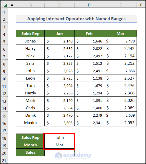
• In cell C20, enter the following formula:

• • The INDIRECT function returns the cell reference of the argument value.

• Press ENTER.

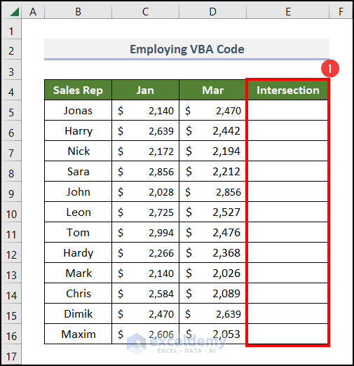
Method 4 – Employing VBA Code

Steps

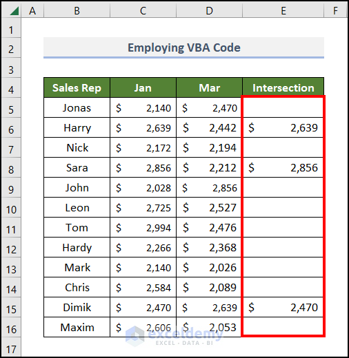
• Create a column with the heading Intersection under Column E (similar to Method 1).

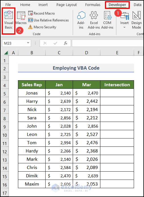
• Go to the Developer tab and click on Visual Basic in the Code group.

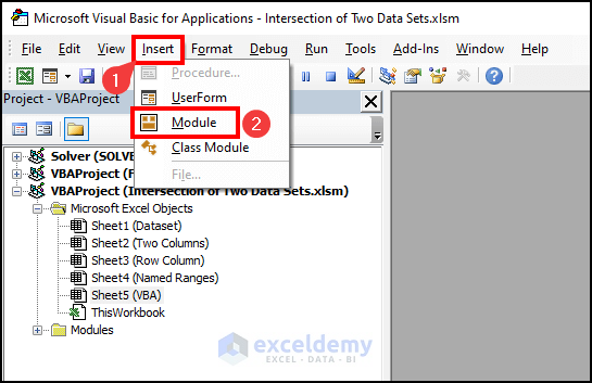
• In the Microsoft Visual Basic for Applications window, go to the Insert tab and select Module.

• Paste the following code into the module:

Sub Intersection_Two_Columns()
Dim Intrsctn As Variant, a As Variant, b As Variant
Set Intrsctn = Range("D5:D16")
For Each a In Selection
For Each b In Intrsctn
If a = b Then a.Offset(0, 2) = a
Next b
Next a
End Sub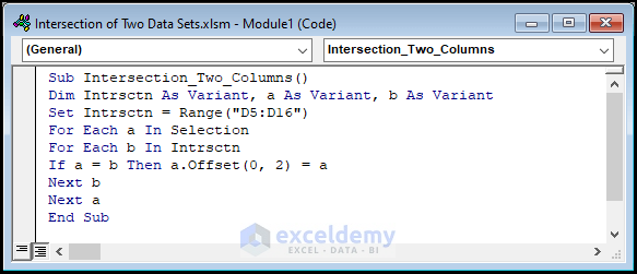

• Save the file as a macro-enabled workbook.
• Select cells in the C5:C16 range (sales in Jan month).
• Navigate to the Developer tab and click on Macros.

• In the Macro dialog box:
  • Select the Intersection_Two_Columns macro in the Macro name box.
  • Click the Run button.

• The output will be the same as Method 1.

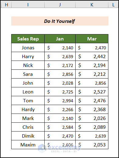
Practice Section

To practice on your own, you’ll find a Practice section similar to the one below on each sheet to the right. Feel free to work through the exercises there.

Download Practice Workbook

You can download the practice workbook from here:

<< Go Back to Excel Operators | Excel Formulas | Learn Excel