Method 1 – Aging Buckets for Overdue Days
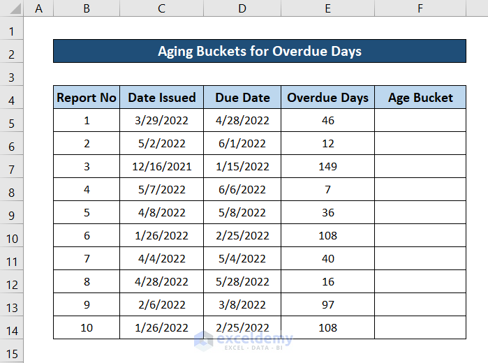
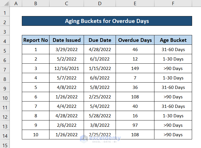
We are going to use the following dataset. It consists of different reports with the dates issued and the due dates. We are going to divide these reports into four buckets: ones that are due for 1-30 days, for 31-60 days, for 61-90 days, and for more than 90 days.
Steps:
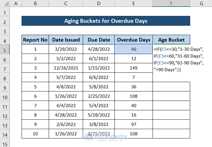
- Select cell F5.
- Copy the following formula in the cell.
=IF(E5<=30,"1-30 Days",IF(E5<=60,"31-60 Days",IF(E5<=90,"61-90 Days",">90 Days")))
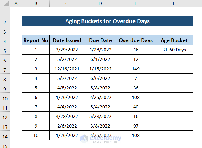
- Press Enter.
- Click and drag the fill handle icon to the end of the column to fill up the rest of the cells with the respective formula.
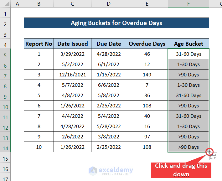
- You will have aging buckets for all the due dates using the IF formula in Excel.
Breakdown of the Formula
IF(E5<=30,”1-30 Days”,IF(E5<=60,”31-60 Days”,IF(E5<=90,”61-90 Days”,”>90 Days”)))
The IF(E5<=30, “1-30 Days”, …) function checks whether the value in cell E5 is true or not. If it is true then the function returns the string written in the second argument. Otherwise, it moves on to the later portion of the formula.
IF(E5<=60, “31-60 Days”, …) checks if the value is smaller or equal to 60 or not. If it is, then it goes to print on the string. Otherwise, it moves on to the next portion of the formula.
IF(E5<=90, “61-90 Days”, “<90 Days”) comes into play if all of the above conditions were false. This function now checks if the value is less than or equal to 90 days or not. If the condition is true, the function returns the string “61-90 Days”. Otherwise, it returns the string “<90 Days”.
Method 2 – Aging Buckets for Number of Days Worked
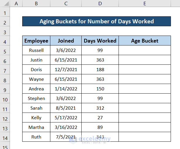
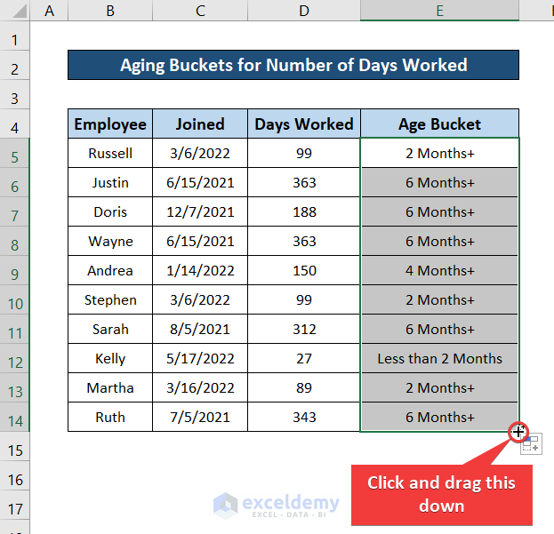
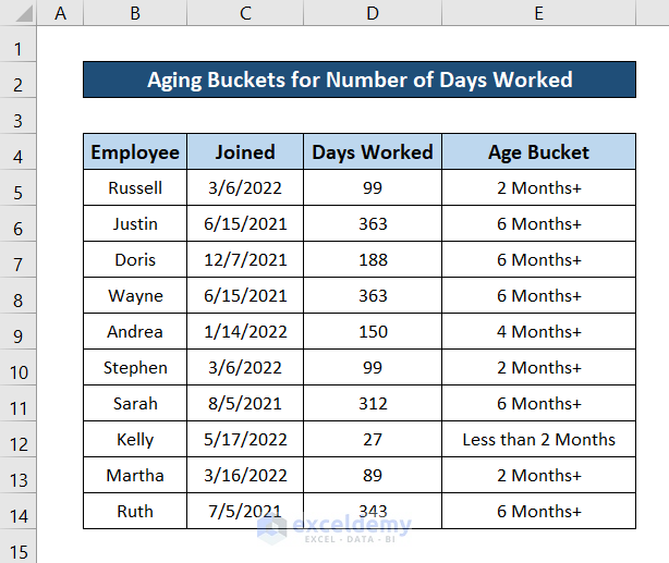
Let’s consider a different dataset like this. This dataset contains a list of employees along with their joining date and the total days they have worked in an organization. Let’s divide them by how long they have worked, and we’ll use four buckets: less than 2 months, more than 2 months, more than 4 months, and longer than 6 months.
Steps:
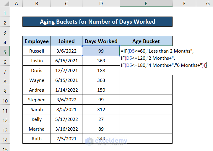
- Select cell E5.
- Copy the following formula in the cell.
=IF(D5<=60,"Less than 2 Months",IF(D5<=120,"2 Months+",IF(D5<=180,"4 Months+","6 Months+")))
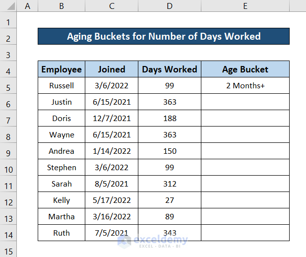
- Press Enter.
- Select the cell again and click and drag the fill handle icon to the end of the column to fill up the rest of the cell with this formula.
- You will have the aging buckets for all the employees depending on the number of days they have worked for.
Breakdown of the Formula
IF(D5<=60,”Less than 2 Months”,IF(D5<=120,”2 Months+”,IF(D5<=180,”4 Months+”,”6 Months+”)))
The IF(D5<=60, “Less than 2 Months”…) function checks whether the value of cell D5 is within 60 or not. If the condition is met, the function goes on to return the string “Less than 2 Months”. Otherwise, it moves on to the next portion of the formula.
If the previous condition is false, the formula moves on to the IF(D5<=120, “2 Months+”,…) portion of the formula. In this section, the function searches whether the value in cell D5 is within 120 now. If the value is indeed within 120, the function returns the string “2 Months+” otherwise it moves on to the next part of the formula.
If all of the conditions above were false, the formula moves on to the IF(D5<=240, “4 Months+”, “6 Months+”) portion. In this portion, the IF function checks for the condition of whether the value in cell D5 is within 240 or not. If the condition is true, the function returns the string “4 Months”. It returns “6 Months” when the condition is false.
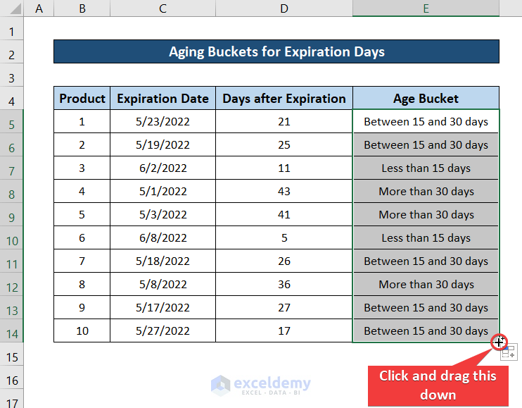
Method 3 – Aging Buckets for Expiration Days
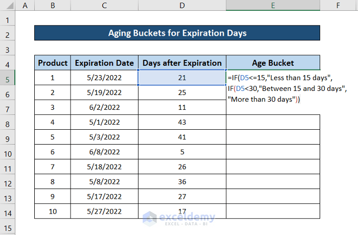
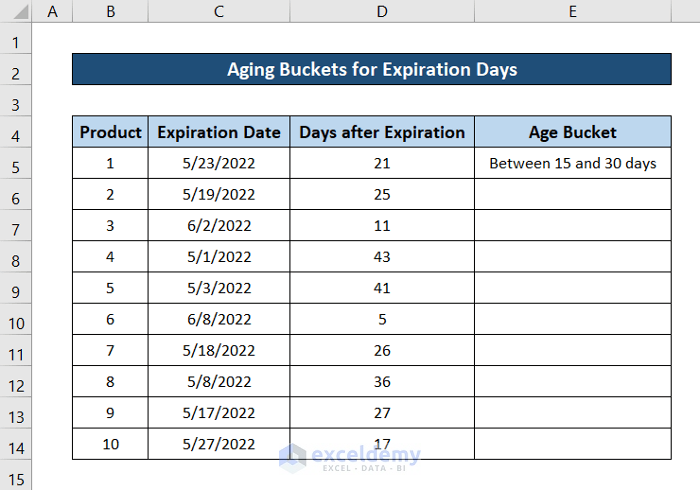
The dataset contains expiration dates for different products. We’ll categorize these products into different aging buckets depending on the number of days after expiration.

Steps:
- Select cell E5.
- Copy the following formula in the cell.
=IF(D5<=15,"Less than 15 days",IF(D5<30,"Between 15 and 30 days","More than 30 days"))
- Press Enter.
- Select the cell and click and drag the fill handle icon to the end of the column to fill out the rest of the cell with this formula.
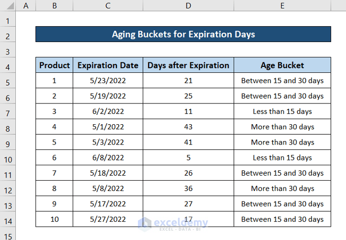
- We will have the aging buckets for all of the entries in the dataset.
Breakdown of the Formula
IF(D5<=15,”Less than 15 days”,IF(D5<30,”Between 15 and 30 days”,”More than 30 days”))
The formula checks for the condition in IF(D5<=15, “Less than 15 days”,…) is true or not. If the formula is true it returns the string in the second argument. When the condition is false, it moves on to the next portion of the formula.
If the above condition is not met, the formula moves on to the IF(D5<30, “Between 15 and 30 days”, “More than 30 days”) portion where it checks for a new condition. It returns the string “Between 15 and 30 days” if this new condition is met. Otherwise, the function returns “More than 30 days”.
Download the Practice Workbook
You can download the workbook containing all the examples used for demonstration in this article from the link below.
<< Go Back to Ageing | Formula List | Learn Excel
Get FREE Advanced Excel Exercises with Solutions!

Hello Sir !
Thanks for the detailed explanation. This has helped me to create age buckets for one of my work activities. But I have a situation. I also have age in negative numbers -1, -2, -3, etc. I need to create to 2 age groups D-30 and D-60. Is it possible using IF formula. Could you please assist.
Really appreciate your help !
Hello MANESH KURKUTE,
Thanks for your response. Yes, we can certainly create the age bucket with negative numbers too. For this, just apply the following formula to have age 0 to -30 to the D-30 Days and -30 to -60 to the D-60 Days.
=IF(C5<= -30,”D-60 Days”,IF(C5<0,”D-30 Days”,IF(C5<=30,”1-30 Days”,IF(C5<=60,”31-60 Days”,IF(C5<=90,”61-90 Days”,”>90 Days”)))))
Regards,
NAIMUL HASAN ARIF
Exceldemy