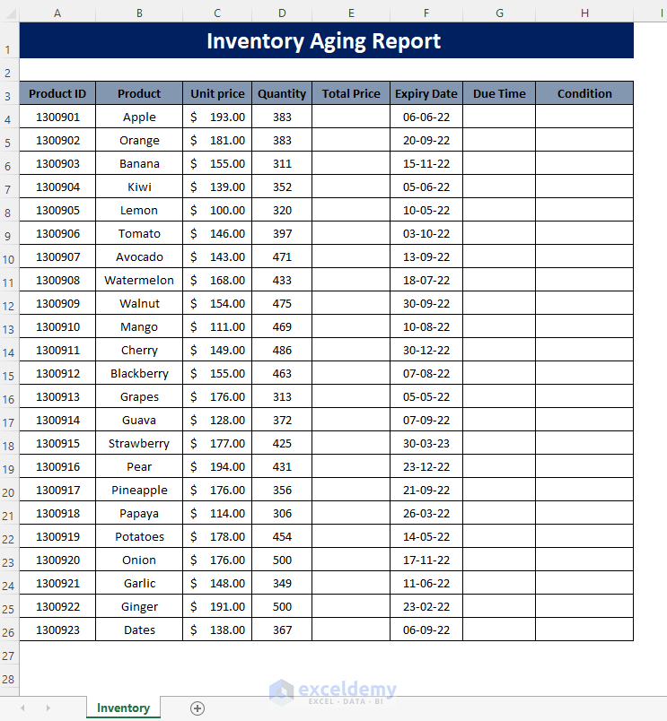
Step 1 – Creating the Basic Outlines
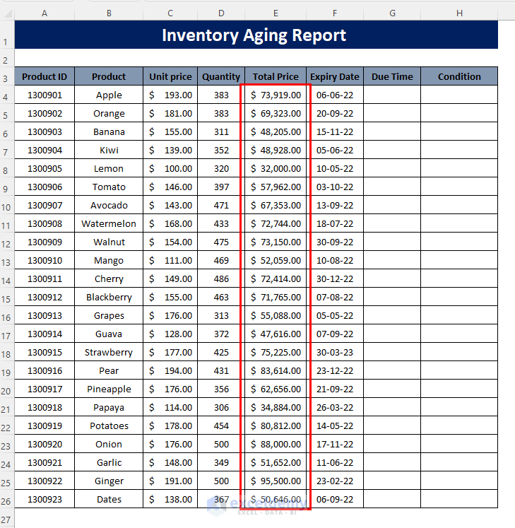
- In the following figure, you can see the basic report for inventory aging and we have created this outline in the Inventory sheet.
- We have the Product IDs, Product names, Unit Prices, Quantities, and Expiry Dates for some of the products.
- Input the values as needed.
- For further calculations, we have inserted three columns: Total Price, Due Time, and Condition.
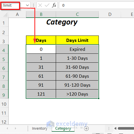
- Create a list showing the categories of the products according to their due times to state the condition or age of the inventories.
- We have also named the range as the limit.
Read More: How to Keep Track of Inventory in Excel
Step 2 – Using Formulas to Make an Inventory Aging Report in Excel
- To calculate the products’ total prices, apply the following formula in cell E4.
=C4*D4C4 is the Unit Price and D4 is the Quantity of the product Apple.
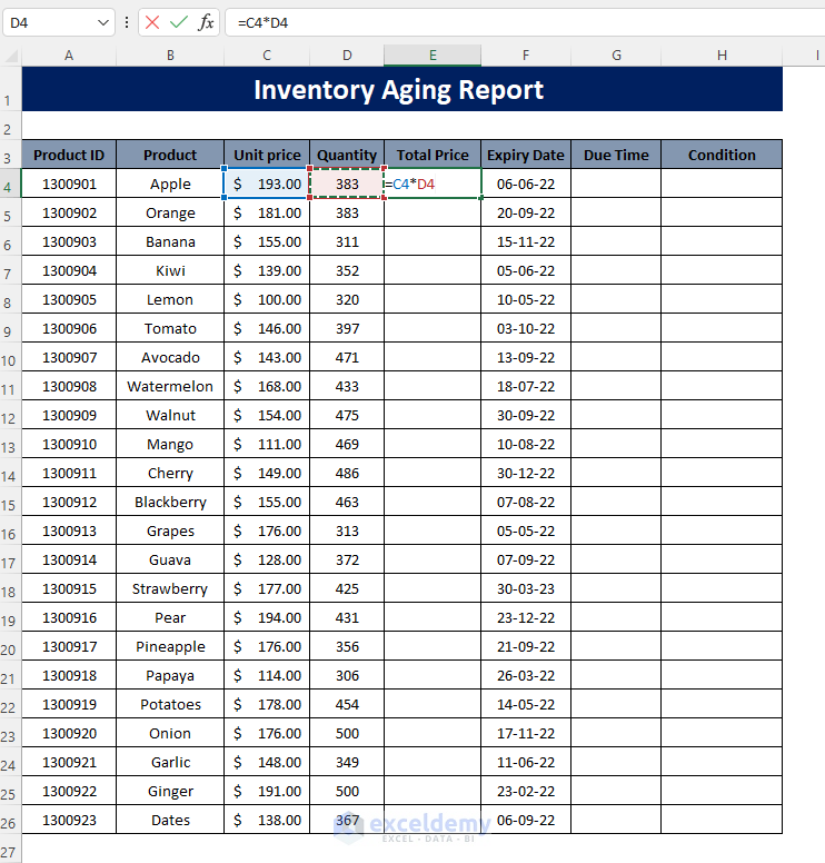
- Press Enter and drag down the Fill Handle tool.
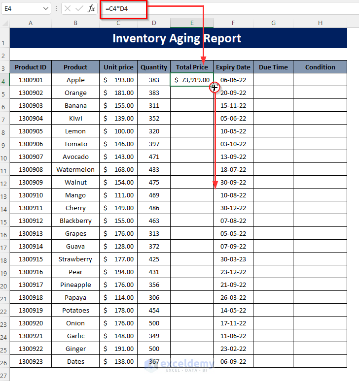
- You will get the total prices for the products in the Total Price column.
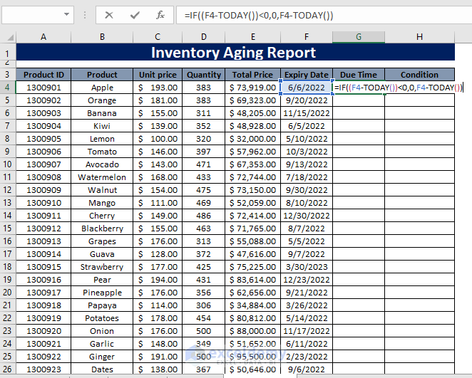
- Calculate the times remaining for the expiration of the products after today’s date with the following formula in G4:
=IF((F4-TODAY())<0,0,F4-TODAY())4 is the Expiry Date of the products, and TODAY() will return today’s date which is 19-05-22.
When the difference between these two values becomes negative IF will return 0 in that case, otherwise for a positive difference value we will get their differences as the Due Time.
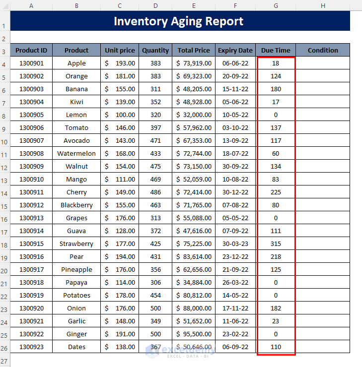
- Press Enter and drag down the Fill Handle tool.
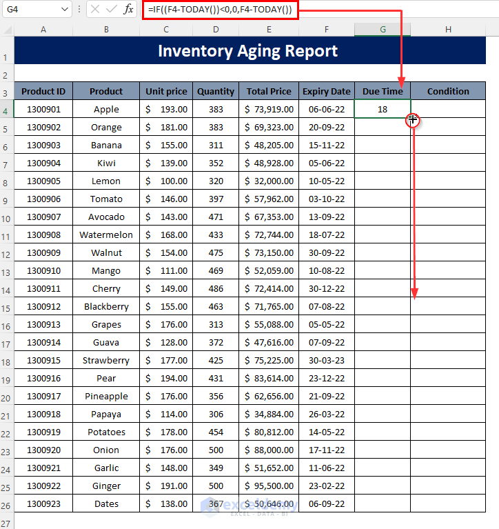
- You will have the due times remaining for the products after today.
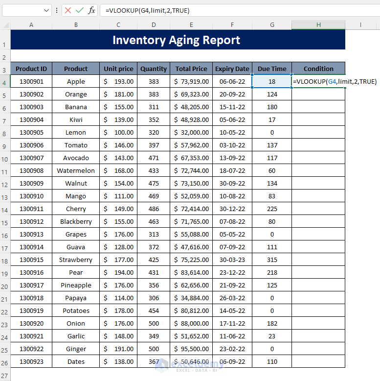
- Put the following formula for checking the condition of the inventory in H4:
=VLOOKUP(G4, limit,2, TRUE)G4 is the look-up value which we are going to look up in the limit named range, 2 is the column index number and TRUE is for an approximate match.
- Press Enter and drag down the Fill Handle tool.
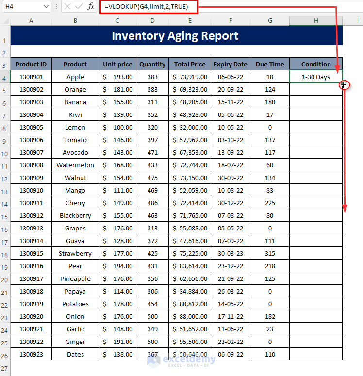
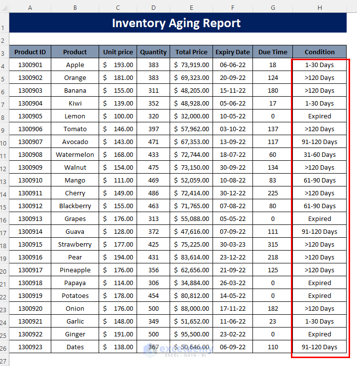
- We will have the conditions of the inventories in the Condition column.
Read More: How to Maintain Store Inventory in Excel
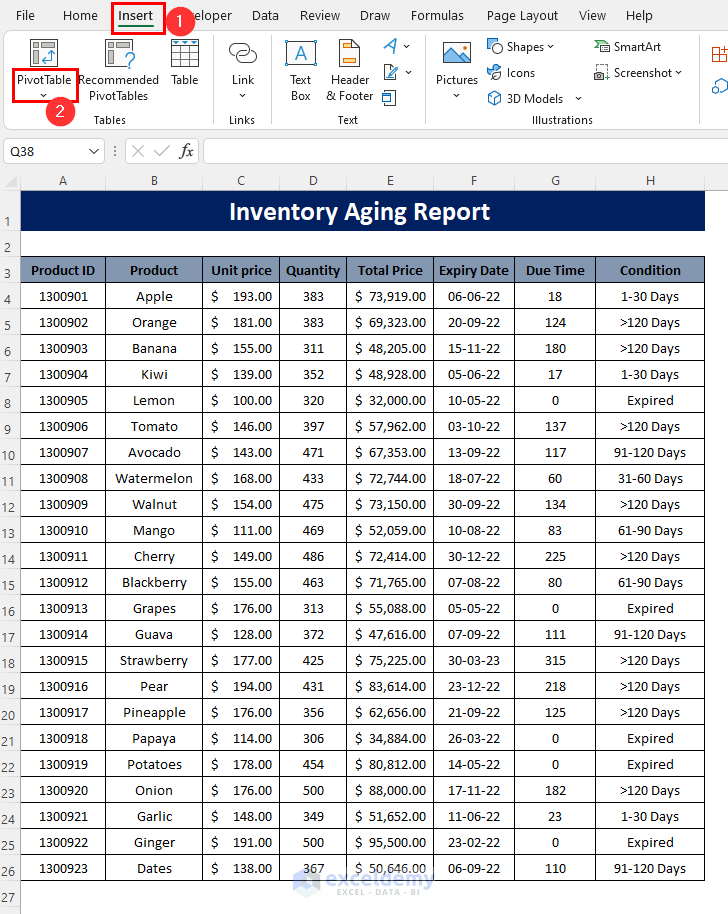
Step 3 – Creating a Pivot Table to Make an Inventory Aging Report
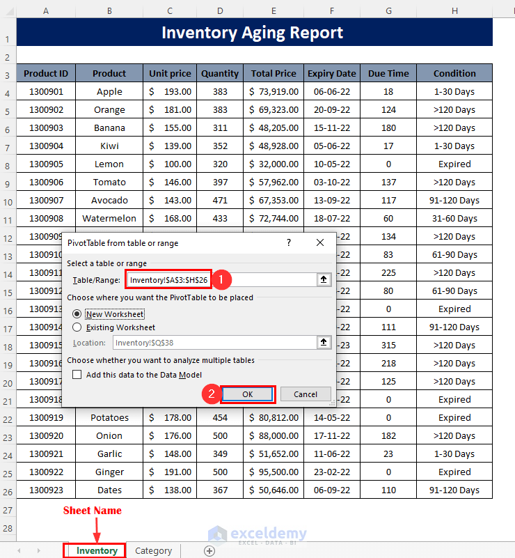
- Go to the Insert tab and select the PivotTable option.
- The PivotTable from table or range dialog box will open up. Select the range of your table from the Inventory sheet and press OK.
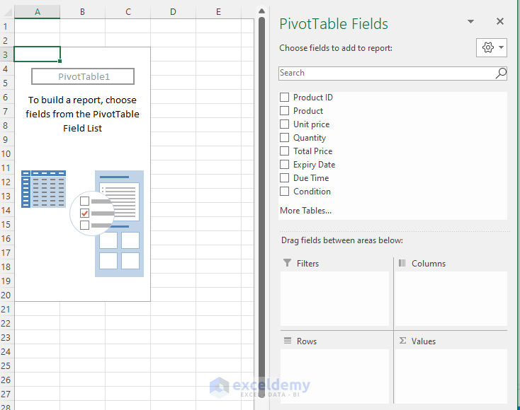
- You will be taken to a new sheet with two portions: PivotTable, and PivotTable Fields.
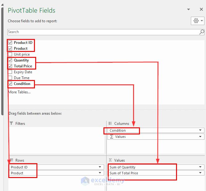
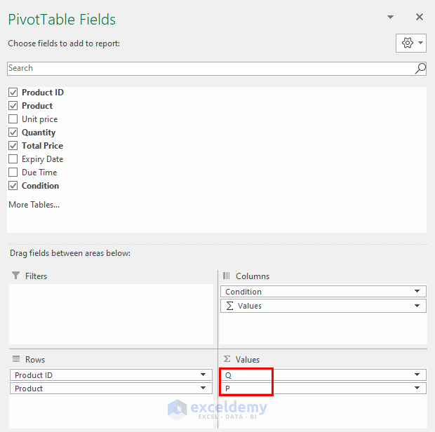
- Drag down the Product ID and Product fields to the Rows area, Quantity and Total Price to the Values area, and Condition to the Columns area.
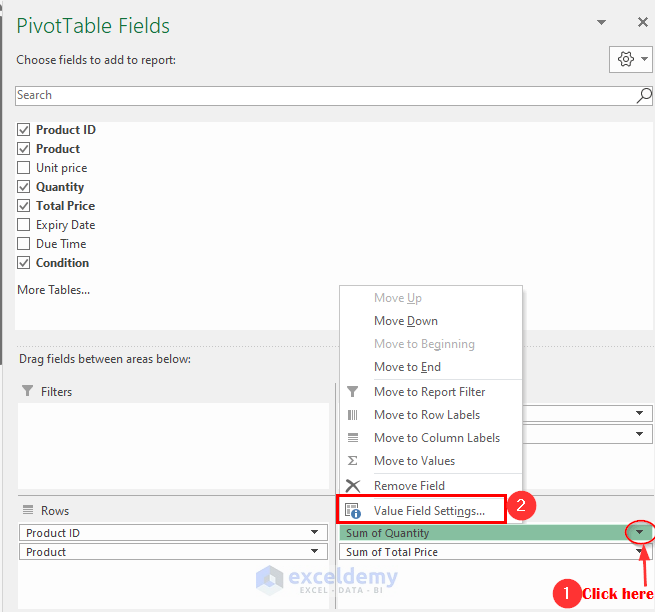
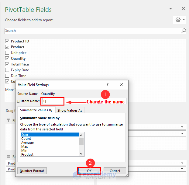
- Click on the dropdown symbol of the Sum of Quantity field and select the option Value Field Settings from different options.
- The Value Field Settings dialog box will open up. Rename the field name as Q or whatever you want in the Custom Name box and press OK.
- Rename the Sum of Total Price field to P for brevity. We are getting the two new field names in the Values area.
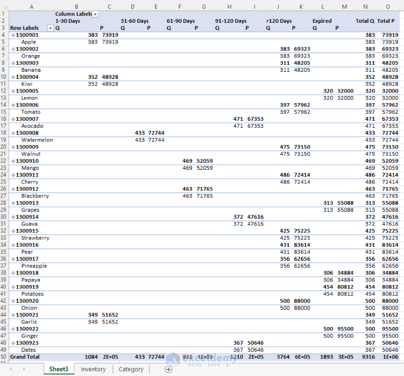
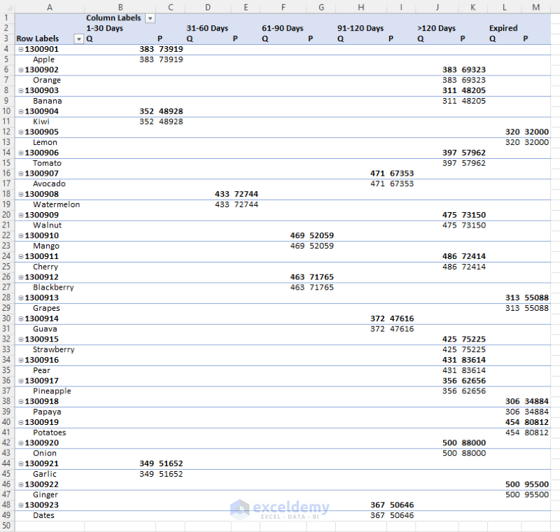
- Here is the pivot table of our data range below with the status of the products as headers of their quantities and prices.
Read More: How to Create Inventory Database in Excel
Step 4 – Formatting the Pivot Table
- Go to the PivotTable Analyze tab and select Options then Options again.
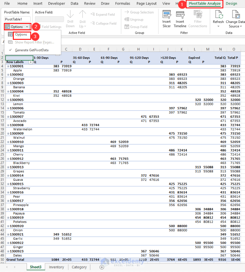
- The PivotTable Options dialog box will open up. Select the Totals & Filters tab and then uncheck the options of the Grand Totals.
- Press OK.
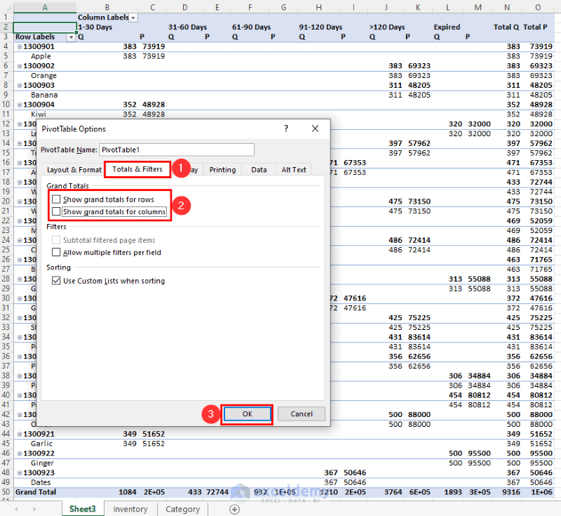
- We have eliminated the total values from the rows and columns.
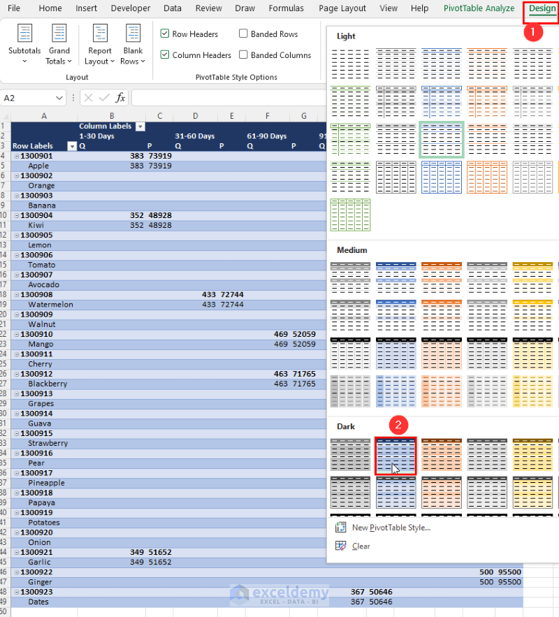
- You can change the design by going to the Design tab and selecting a theme.
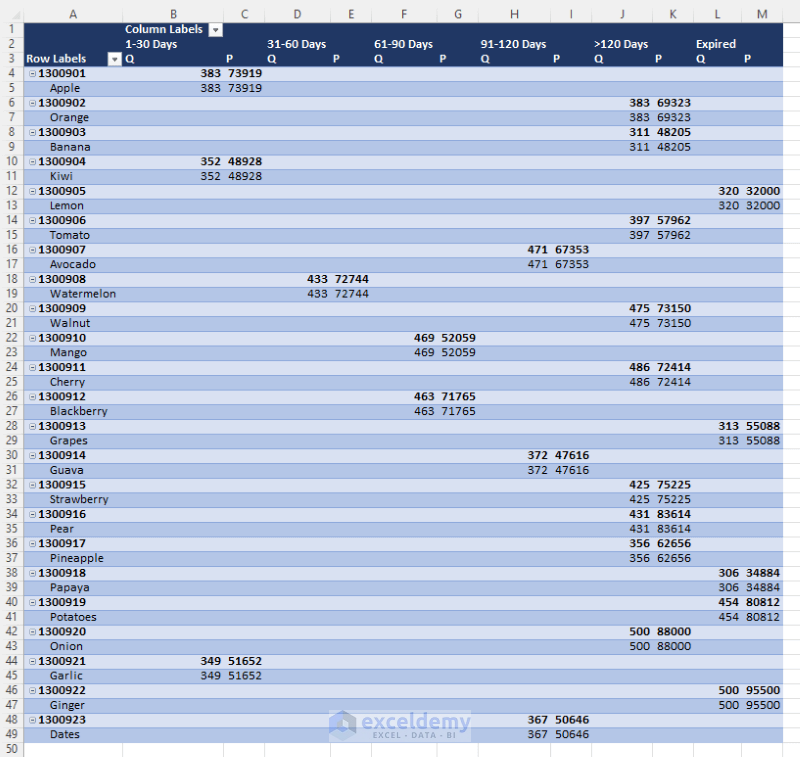
- Here is the final look of our Inventory Aging Report.
Download the Workbook
Related Articles
- Min Max Inventory Calculation in Excel
- How to Calculate Economic Order Quantity in Excel
- How to Calculate Stock to Sales Ratio Using Formula in Excel
<< Go Back to Inventory Management in Excel | Learn Excel
Get FREE Advanced Excel Exercises with Solutions!
